Matching the Statistical Query Lower Bound for $k$-Sparse Parity Problems with Sign Stochastic Gradient Descent

EbSSBvwUWw

Yiwen Kou et el.

TL;DR
#

The k-sparse parity problem is a significant benchmark in computational complexity, posing a challenge to efficiently learn functions in high-dimensional spaces. Existing methods either fell short of established Statistical Query (SQ) lower bounds or required computationally expensive approaches. This problem relates to understanding P vs NP and is vital in error correction, information theory, and many other areas.

This research demonstrates that a relatively simple method—sign stochastic gradient descent (SGD) applied to two-layer neural networks—can efficiently solve the k-sparse parity problem. The algorithm achieves a sample complexity of Õ(dk−1), directly matching the established SQ lower bounds. This is a significant advancement, as it shows that computationally tractable gradient-based methods can indeed reach theoretical optima, providing important insight for machine learning algorithm design and analysis.

Key Takeaways
#

Why does it matter?
#

This paper is crucial because it bridges the gap between theoretical lower bounds and practical algorithm performance in learning sparse parity problems. It offers a computationally efficient method using sign SGD, which has significant implications for the broader field of machine learning, particularly in scenarios involving high-dimensional data with sparse structure. This opens up new avenues for research into the theoretical understanding of gradient descent and its practical applications.

Visual Insights
#

🔼 The figure compares the standard sign function with a modified version that includes a dead zone. In the modified sign function, there is a region around zero where the output is zero, creating a threshold effect. The standard sign function outputs +1 for any positive input and -1 for any negative input.
read the caption
Figure 1: The plot above illustrates the comparison between the modified sign function sign(x)(p = 0.5) and the standard sign function sign(x). The sign(x) function introduces a ‘dead zone' between -p and p where the function value is zero, which is not present in the standard sign function. This modification effectively creates a threshold effect, only outputting non-zero values when the input x exceeds the specified bounds of p in either direction.

🔼 This table compares various existing works on solving the XOR (2-parity) problem using neural networks. It contrasts different activation functions, loss functions, algorithms (e.g., gradient flow, SGD), width requirements of the neural network, sample complexity, and the number of iterations required to converge. The table highlights the dependence of these parameters on the input dimension (d) and the test error (e). It specifically notes that the sample and iteration requirements for both Glasgow’s (2023) method and the authors’ method are implicitly dependent on the test error (e), and it details the specific conditions on the dimension (d) that must be met for each.
read the caption
Table 1: Comparison of existing works on the XOR (2-parity) problem. We mainly focus on the dependence on the input dimension d and test error e and treat other arguments as constant. Here WF denotes Wasserstein flow technique from the mean-field analysis, and GF denotes gradient flow. The sample requirement and convergence iteration in both Glasgow (2023) and our method do not explicitly depend on the test error €. Instead, the dependence on e is implicitly incorporated within the condition for d. Specifically, our approach requires that d > C log²(2m/e) while Glasgow (2023) requires d > exp((1/6)C) where C is a constant.

In-depth insights
#

Sign SGD’s Power
#

SignSGD’s power lies in its ability to achieve comparable performance to full-precision SGD while significantly reducing computational costs. By utilizing only the sign of the gradient, SignSGD decreases memory usage and communication overhead, making it particularly attractive for large-scale distributed training. The algorithm’s robustness to noise is another key advantage, allowing it to efficiently navigate the complex optimization landscape of deep neural networks. The theoretical analysis in this paper shows that SignSGD matches the established statistical query lower bound for solving k-sparse parity problems, a challenging benchmark in learning theory, demonstrating its effectiveness in handling high-dimensional data. Its computational efficiency, coupled with its robustness and theoretical guarantees, positions SignSGD as a powerful tool for training complex models, particularly when resources are limited. Further exploration of SignSGD’s applicability in various machine learning tasks and different network architectures warrants further research.

Parity Problem Solved
#

A research paper claiming to have “solved” the parity problem likely makes a significant contribution to theoretical computer science and machine learning. The parity problem, particularly in its sparse variant, is a benchmark problem for understanding the computational limits of various learning models. A claimed solution would likely involve a novel algorithm or approach, possibly leveraging advanced mathematical techniques or insights from neural network architectures. The significance would depend heavily on the efficiency and scalability of the proposed solution. If the solution achieves optimal or near-optimal performance with respect to known lower bounds, it would be exceptionally impactful. However, the term “solved” should be carefully considered. A complete solution may imply achieving a provably correct algorithm that surpasses existing approaches in efficiency, error rate, and applicability, while a partial solution might focus on specific problem instances or utilize specific assumptions. Regardless, any claimed solution to the parity problem would warrant close examination for its innovative methods, theoretical rigor, and practical implications for various computational domains.

Network Architecture
#

The research paper’s core methodology centers on a two-layer fully-connected neural network, a relatively simple architecture. This choice is deliberate; it allows for a clear analysis of the algorithm’s performance without being hampered by the complexities of deeper networks. The network’s simplicity facilitates a rigorous theoretical analysis, permitting the authors to establish a direct link between the network’s properties and its capacity to solve the k-sparse parity problem. The use of a polynomial activation function within the architecture is a non-standard choice, but it plays a vital role in the theoretical analysis, which is tailored to the specific properties of this activation function. The relatively narrow width of the network, scaled to 2^k where k represents the sparsity parameter, is also notable. This width, while seeming exponential in k, is independent of the input dimension d. The sign SGD training method interacts significantly with the architecture; its convergence properties are heavily reliant on the polynomial activation and the network’s specific structure. The combination of these components—network architecture, activation function, and training algorithm—forms a powerful yet analytically tractable system for studying the limits of SGD in solving parity problems.

Limitations of SGD
#

Stochastic Gradient Descent (SGD), while a powerful optimization algorithm, exhibits limitations relevant to the k-sparse parity problem. Sign-SGD’s reliance on gradient normalization might hinder performance in non-standard or unknown coordinate systems. This suggests exploring adaptive learning rates or momentum-based methods. The theoretical analysis heavily relies on polynomial activation functions, limiting generalizability to other activation functions like ReLU or sigmoid. Approximating these functions using polynomials introduces errors, impacting overall accuracy and requiring careful assessment of approximation error. Furthermore, the batch size requirements in Sign-SGD scale exponentially with k, potentially becoming computationally expensive for large k values. Finally, while the theoretical analysis matches the statistical query lower bound for a standard k-sparse parity problem, empirical validation of the theoretical findings is crucial, providing a critical next step in understanding the performance limits and potential generalizability of the approach.

Future Research
#

The paper’s “Future Research” section could explore extending the current work on k-sparse parity problems to more complex scenarios. Investigating alternative optimization algorithms beyond sign SGD, such as Adam or other adaptive methods, could reveal performance improvements. Addressing scenarios with non-isotropic data distributions is crucial, as the current analysis relies on uniform data, which might not reflect real-world datasets. Another promising avenue would be exploring the impact of different neural network architectures, going beyond the two-layer fully-connected model used in this work. Finally, a deeper theoretical analysis is needed to provide a comprehensive understanding of the algorithm’s behavior, potentially providing tighter bounds on sample complexity or clarifying the role of specific hyperparameters. These avenues promise valuable insights into the broader applicability and limitations of the proposed approach.

More visual insights
#

More on figures

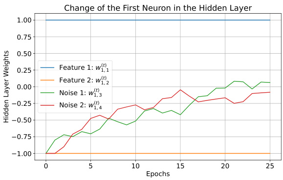
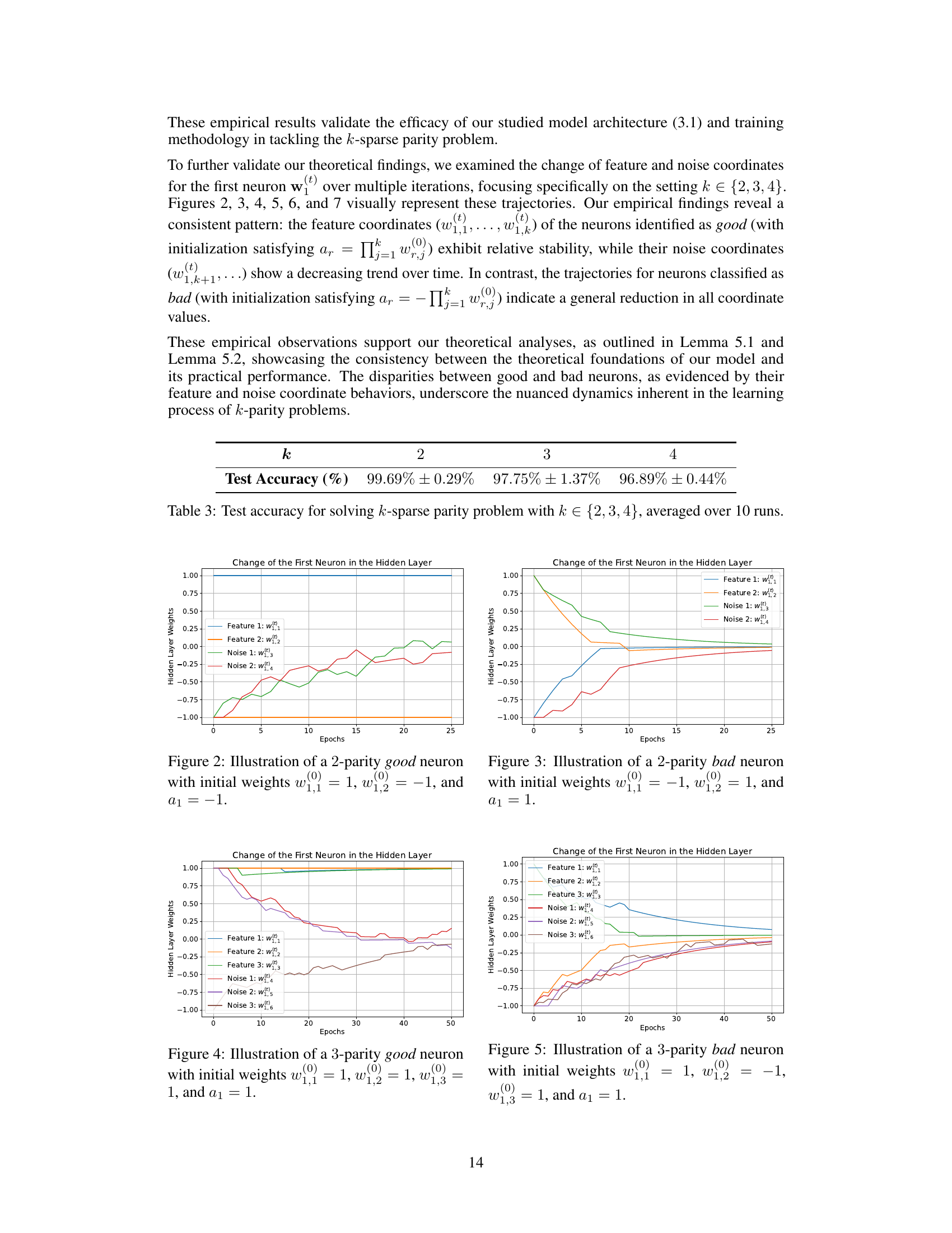
🔼 This figure shows the change of weights of a single neuron in a two-layer neural network over 25 epochs while training on a 2-parity problem. The neuron is categorized as a ‘good’ neuron based on its initialization. The plot displays the trajectories of the weights associated with the two features (w_1,1^(t) and w_1,2^(t)) and the two noise coordinates (w_1,3^(t) and w_1,4^(t)) of the neuron. The plot demonstrates how the feature weights remain relatively stable over time, while the noise weights decay to a magnitude of almost zero.
read the caption
Figure 2: Illustration of a 2-parity good neuron with initial weights w_1,1⁽⁰⁾ = 1, w_1,2⁽⁰⁾ = -1, and a₁ = -1.

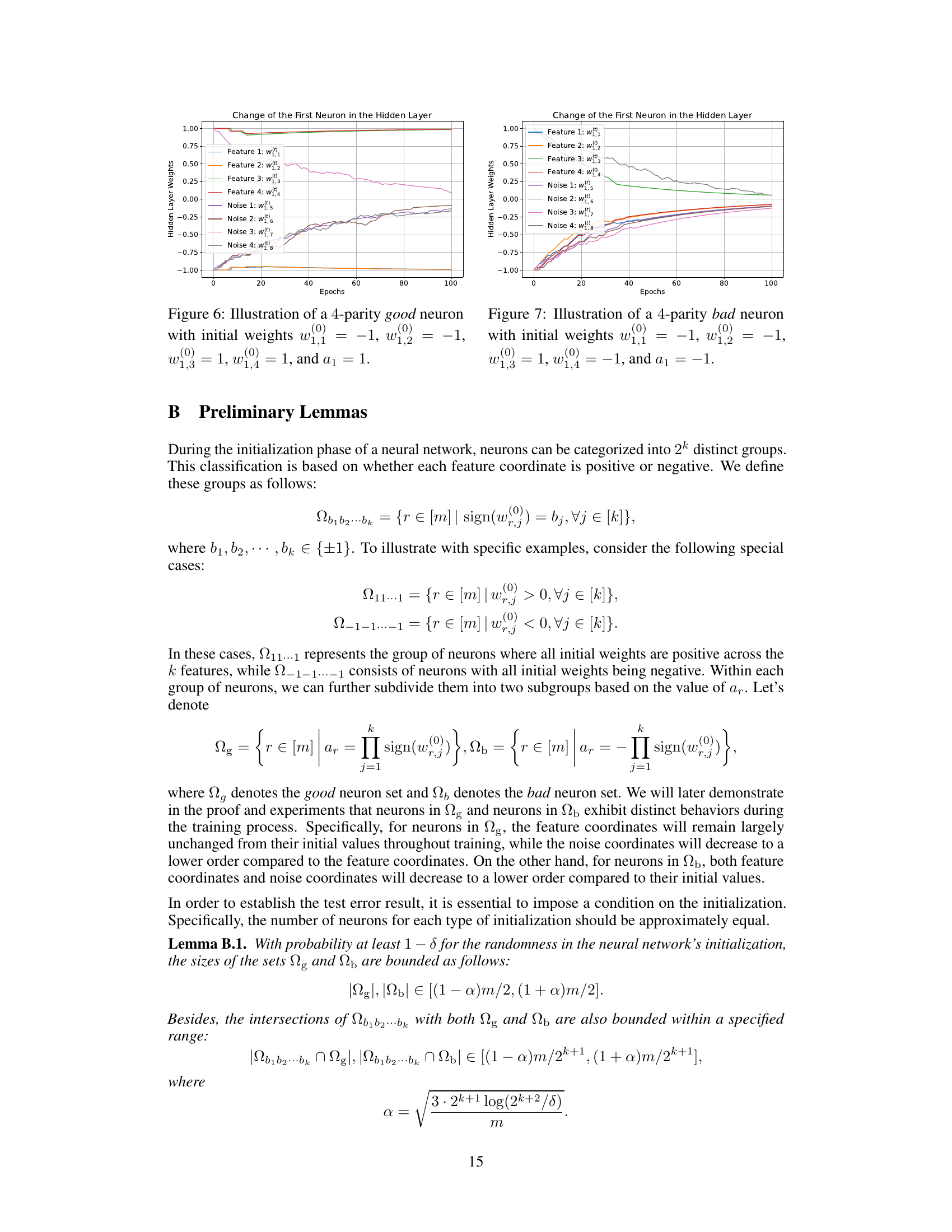
🔼 This figure shows the change in the weights of a single neuron in a two-layer neural network trained with sign SGD to solve the 2-parity problem over 25 epochs. The neuron is considered ‘good’ because its initial weights and second-layer weight (a₁) have a specific configuration that aligns well with the solution. The plot displays the change in the weights associated with the two features (w_1,1 and w_1,2) and two noise dimensions (w_1,3 and w_1,4) of the neuron. The graph shows that the feature weights (w_1,1 and w_1,2) remain relatively stable during training, while the noise weights (w_1,3 and w_1,4) decrease to near zero, demonstrating that sign SGD effectively filters out noise dimensions during training.
read the caption
Figure 2: Illustration of a 2-parity good neuron with initial weights w_1,1⁽⁰⁾ = 1, w_1,2⁽⁰⁾ = -1, and a₁ = -1.

🔼 This figure shows the change of the first neuron’s weights in a hidden layer during the training process for a 2-parity problem. The neuron is categorized as a ‘good’ neuron because its initial weights align with the true solution. The plot displays the weights of feature coordinates (w(t)1,1 and w(t)1,2) and noise coordinates (w(t)1,3, w(t)1,4, w(t)1,5, and w(t)1,6) over epochs. The feature coordinates remain relatively stable, indicating their alignment with the parity function. Conversely, the noise coordinates decay exponentially, illustrating their insignificance in the solution.
read the caption
Figure 2: Illustration of a 2-parity good neuron with initial weights w(0)1,1 = 1, w(0)1,2 = -1, and a1 = -1.

🔼 This figure shows the change in weights of a 2-parity good neuron over epochs. A good neuron is one where the initial weights align with the correct parity. In this example, the feature weights (w(t)1,1 and w(t)1,2) remain relatively stable, while the noise weights (w(t)1,3 and w(t)1,4) decrease to near zero over time. This illustrates the efficient learning and denoising characteristics of sign SGD for good neurons.
read the caption
Figure 2: Illustration of a 2-parity good neuron with initial weights w(0)1,1 = 1, w(0)1,2 = -1, and a1 = -1.

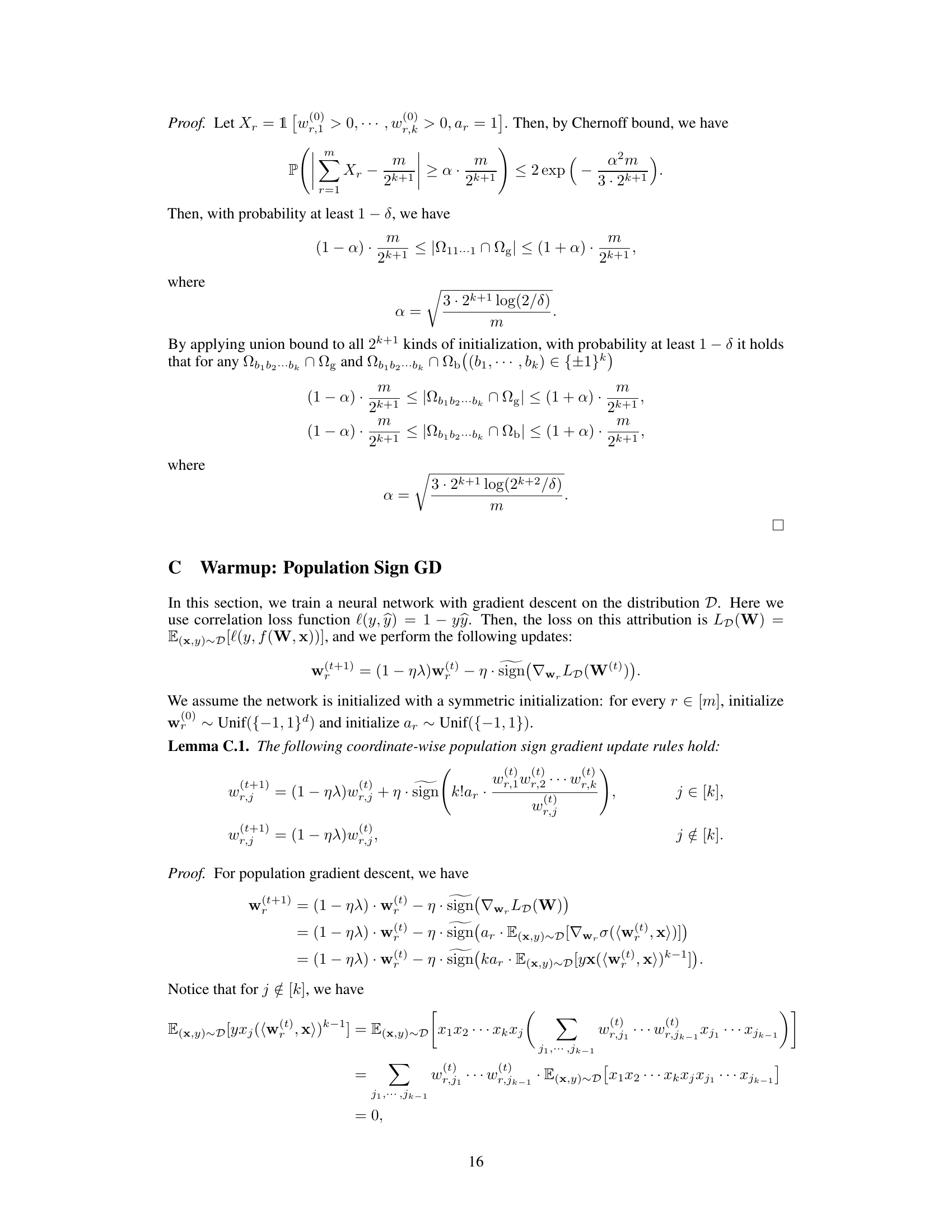
🔼 This figure shows the change in weights of a 4-parity bad neuron over training epochs. The neuron is classified as ‘bad’ due to its initial weight configuration and resulting behavior. The plot illustrates how the feature weights (w1,1 to w1,4) and noise weights (w1,5 to w1,8) evolve during training, demonstrating the characteristic decay observed in bad neurons.
read the caption
Figure 7: Illustration of a 4-parity bad neuron with initial weights w(0)1,1 = −1, w(0)1,2 = −1, w(0)1,3 = 1, w(0)1,4 = −1, and a1 = −1.

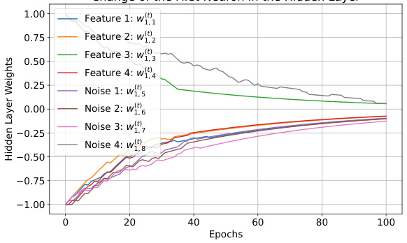
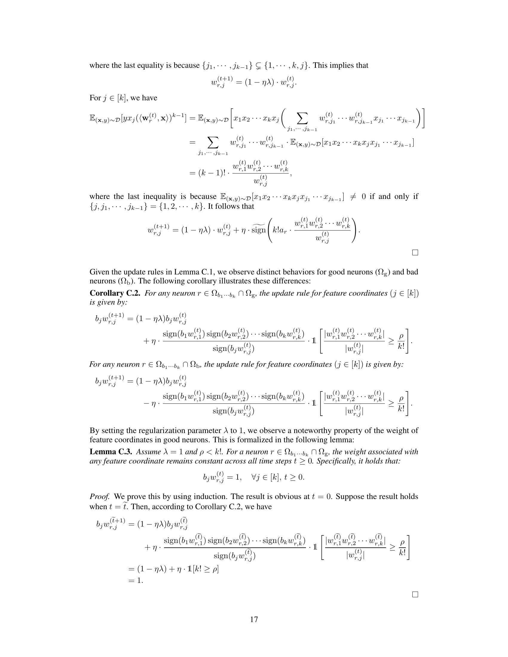
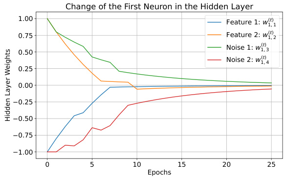
🔼 This figure shows the trajectory of weights of a 4-parity bad neuron during training. The neuron’s initial weights are w1,1(0) = −1, w1,2(0) = −1, w1,3(0) = 1, w1,4(0) = −1, and its second layer weight is a1 = −1. The plot illustrates how the weights of feature coordinates and noise coordinates change over epochs (iterations). The x-axis represents epochs of training, and the y-axis represents the value of the weights. As this is a bad neuron, all weights tend towards 0, indicating that the neuron does not effectively contribute to learning the 4-parity function. In contrast to a good neuron, where feature weights maintain their initial values and noise weights tend to 0, a bad neuron’s weights all gradually approach zero, demonstrating that this neuron does not learn the target function.
read the caption
Figure 7: Illustration of a 4-parity bad neuron with initial weights w1,1(0) = −1, w1,2(0) = −1, w1,3(0) = 1, w1,4(0) = −1, and a1 = −1.

TL;DR#

Key Takeaways#

Why does it matter?#

Visual Insights#

In-depth insights#

Sign SGD’s Power#

Parity Problem Solved#

Network Architecture#

Limitations of SGD#

Future Research#

More visual insights#

Full paper#