TL;DR#
Adaptive optimization methods are crucial in machine learning due to their efficiency in learning rate tuning. However, existing methods like AdaGrad suffer from performance degradation when dealing with poorly scaled data. This paper addresses this issue by proposing a novel algorithm.
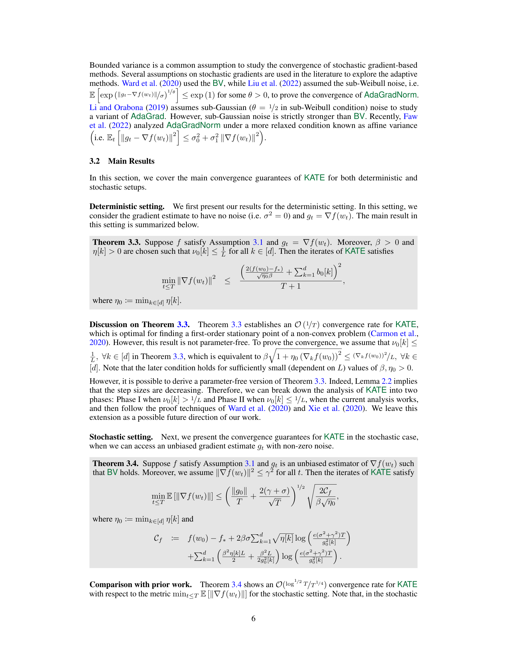
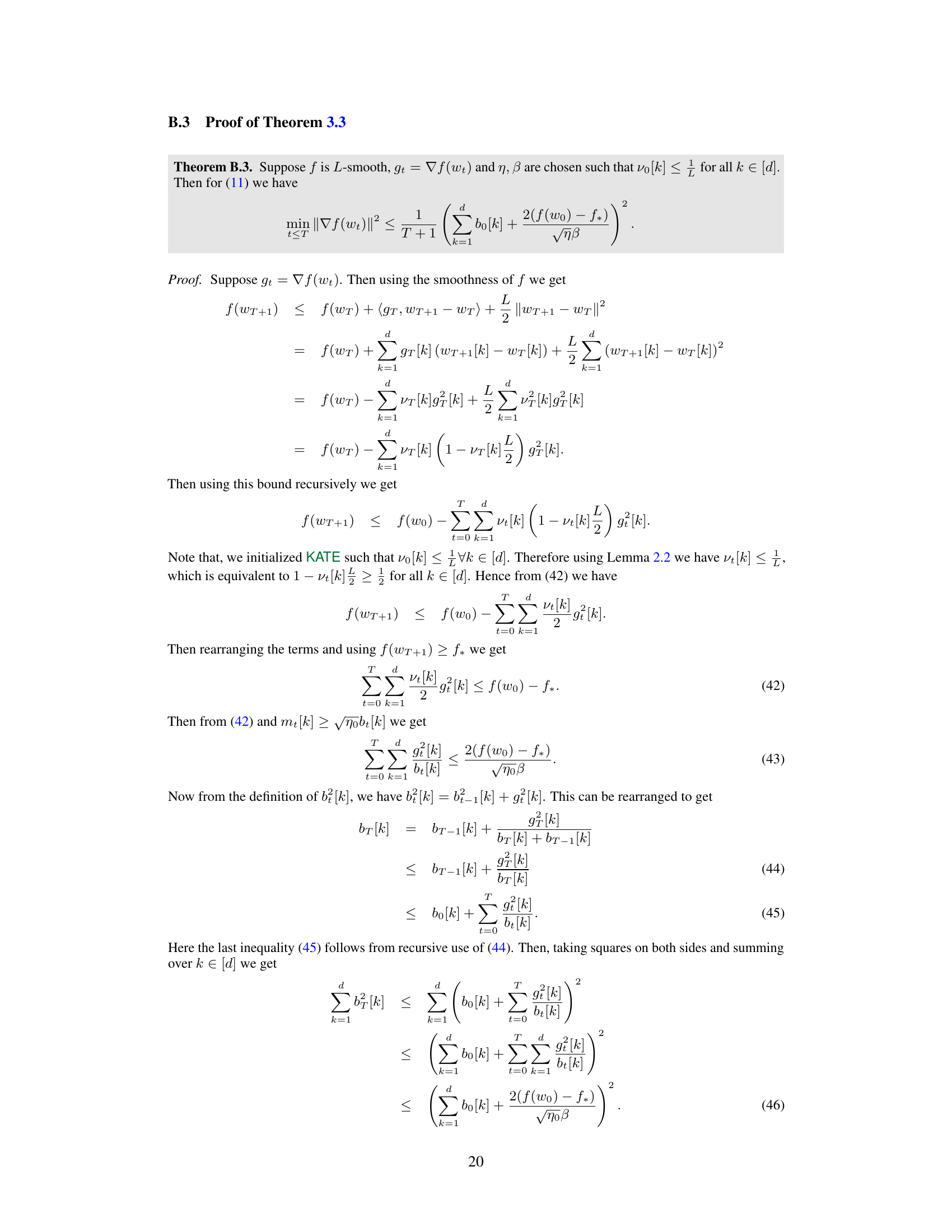
The paper introduces KATE, a scale-invariant version of AdaGrad. Unlike AdaGrad, KATE doesn’t use a square root in its step-size calculation, improving robustness to data scaling. The authors theoretically prove KATE’s scale-invariance for generalized linear models and establish its convergence rate, matching state-of-the-art algorithms. Extensive experiments across various machine learning tasks demonstrate that KATE outperforms AdaGrad and is comparable or superior to Adam.
Key Takeaways#
Why does it matter?#
This paper is important because it introduces KATE, a novel scale-invariant optimization algorithm that addresses the limitations of AdaGrad. Its proven convergence rate and superior performance in various machine learning tasks make it a valuable tool for researchers, opening avenues for improved model training and potentially impacting diverse applications.
Visual Insights#

🔼 This figure compares the performance of KATE against four other algorithms (AdaGrad, AdaGradNorm, SGD-decay, and SGD-constant) on a logistic regression task. It demonstrates KATE’s robustness across various initializations (represented by Δ). The plots illustrate the functional value, accuracy, and gradient norm after different numbers of iterations, highlighting KATE’s efficiency and stability compared to the other methods.
read the caption
Figure 1: Comparison of KATE with AdaGrad, AdaGradNorm, SGD-decay and SGD-constant for different values of ∆ (on x-axis) for logistic regression model. Figure 1a, 1b and 1c plots the functional value f (wt) (on y-axis) after 104, 5 × 10⁴, and 105 iterations respectively.
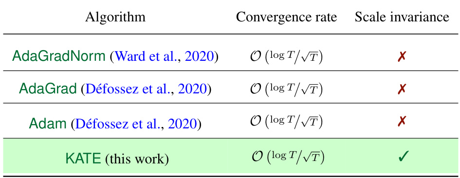
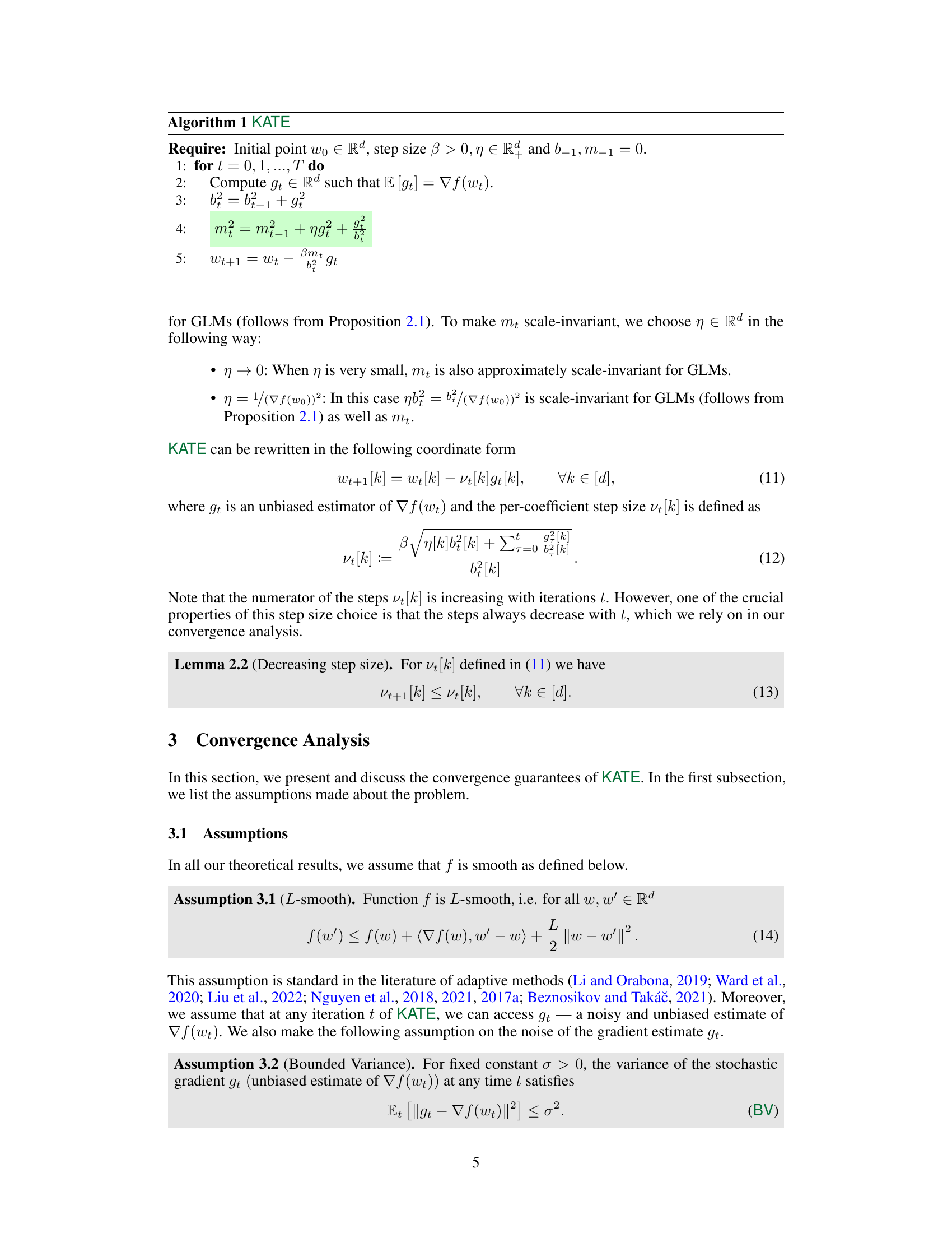
🔼 The table summarizes the convergence rates and scale invariance properties of several adaptive optimization algorithms, including AdaGradNorm, AdaGrad, Adam, and the newly proposed KATE algorithm. It shows that KATE achieves a convergence rate comparable to the others (O(log T/√T)) but is uniquely scale-invariant.
read the caption
Table 1: Summary of convergence guarantees for closely-related adaptive algorithms to solve smooth non-convex stochastic optimization problems. Convergence rates are given in terms of mint∈[T] E [||∇f(wt)||]². We highlight KATE's scale-invariance property for problems of type (4).
In-depth insights#
KATE: Scale Invariance#
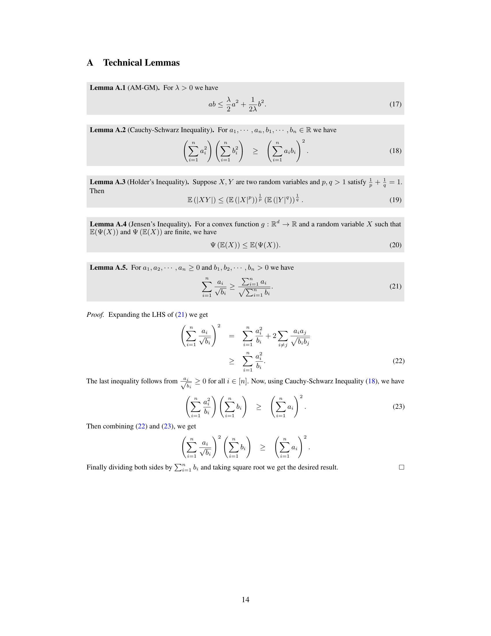
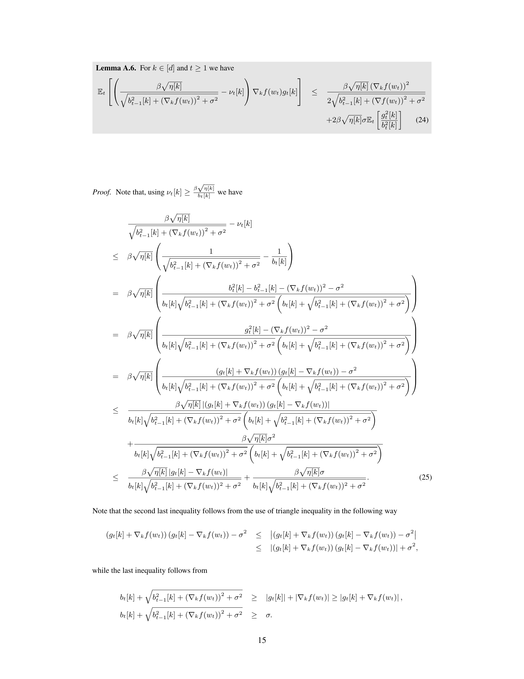
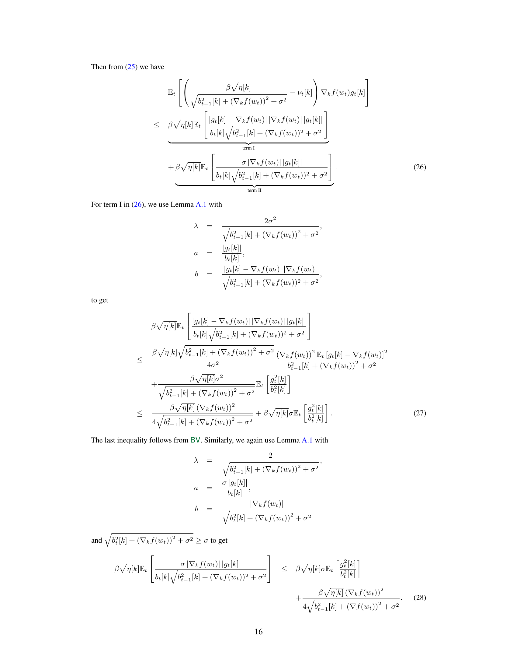
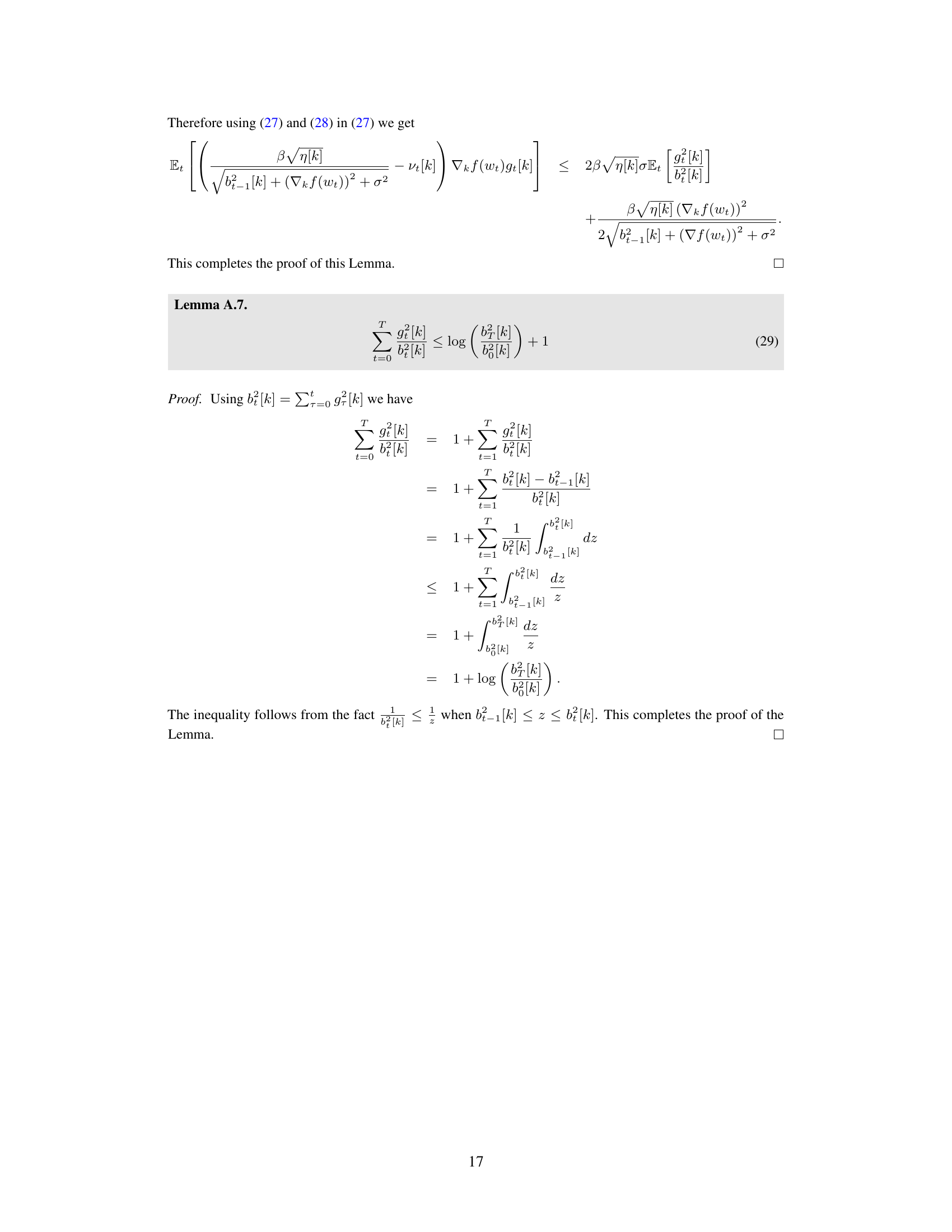
The concept of “KATE: Scale Invariance” centers on addressing a critical limitation of AdaGrad, its sensitivity to data scaling. KATE (Kernel Adaptive and Tuneable Estimator) introduces a novel approach by removing the square root from the denominator of the AdaGrad step size. This modification, combined with a carefully designed numerator sequence, achieves scale invariance. This means KATE’s performance remains consistent regardless of how the input data is scaled, unlike AdaGrad which can significantly underperform with poor scaling. The paper proves this scale invariance property for Generalized Linear Models, a widely applicable class of models, and demonstrates experimentally its robustness across various machine learning tasks. The theoretical convergence rate analysis provides further support, showing that KATE’s performance matches or surpasses that of other adaptive algorithms like Adam in multiple scenarios. This scale-invariance is a crucial advantage, especially for real-world applications where data preprocessing and careful scaling often proves to be a major challenge.
AdaGrad’s limitations#
AdaGrad, despite its early success, suffers from significant limitations. Its primary weakness is its dependence on a decaying learning rate, which becomes increasingly small as training progresses. This can severely hinder performance on large datasets or those with complex structures, as the algorithm may not sufficiently explore the parameter space before convergence. Another critical limitation is its sensitivity to feature scaling. The algorithm’s performance can degrade considerably if features have drastically different scales, leading to suboptimal results. The square root operation in the AdaGrad update rule can also be computationally expensive, especially for high-dimensional data, making it less efficient compared to other adaptive methods. Furthermore, AdaGrad struggles in non-convex optimization settings, where its convergence guarantees are weaker and its performance can be inconsistent. Finally, the requirement of storing the sum of squared gradients can lead to a significant memory footprint, a considerable barrier for large-scale problems.
Convergence Analysis#
The convergence analysis section of a research paper is crucial for validating the effectiveness of a proposed algorithm. A thorough analysis would typically begin by stating the assumptions made about the problem, such as the smoothness or convexity of the objective function. These assumptions define the scope of the results. Then, the analysis would delve into proving convergence rates, ideally establishing tight bounds on how quickly the algorithm approaches a solution. For non-convex problems, the analysis might focus on convergence to stationary points or satisfying specific optimality conditions. It’s essential to consider different scenarios including deterministic and stochastic settings, acknowledging the impact of noise on convergence. A robust analysis would also include comparisons with existing algorithms, highlighting improvements in convergence speed or other key metrics. Finally, a discussion of the limitations of the analysis and its implications for practical application would add value and show a complete understanding of the work.
Empirical Evaluation#
An empirical evaluation section in a research paper should meticulously detail experiments to validate the proposed method. It should include a clear description of datasets used, outlining their characteristics and relevance. The evaluation metrics must be explicitly stated and justified, and any preprocessing steps applied to the data should be transparently documented. Benchmarking against existing state-of-the-art methods is crucial for establishing the novelty and effectiveness of the new approach. The results should be presented clearly, ideally with visualizations like graphs or tables, indicating performance scores and highlighting key differences between approaches. Statistical significance testing should be performed to rule out random chance as a factor in observed performance gains. Error bars or confidence intervals should be presented along with any statistical tests conducted. The section should also discuss potential limitations of the experimental setup and any unexpected results observed. A thorough analysis will provide robust evidence supporting the paper’s claims.
Future Research#
Future research directions stemming from this work could involve extending the theoretical analysis to broader classes of optimization problems, moving beyond the current focus on smooth non-convex functions and exploring settings with less restrictive assumptions on the noise and variance of the stochastic gradients. Another promising avenue would be to investigate the performance of KATE in high-dimensional settings, such as those encountered in deep learning, where the computational cost of adaptive methods can become a significant bottleneck. Additionally, developing a more principled method for selecting the hyperparameter η would be beneficial, potentially through adaptive strategies or techniques that learn the optimal value from the data itself. Further research might also explore combinations of KATE with other optimization techniques, such as momentum methods or variance reduction approaches, to further improve performance and efficiency. Finally, a thorough empirical comparison of KATE against a broader range of adaptive algorithms on diverse machine learning tasks would strengthen the findings and provide a more complete understanding of its capabilities and limitations.
More visual insights#
More on figures
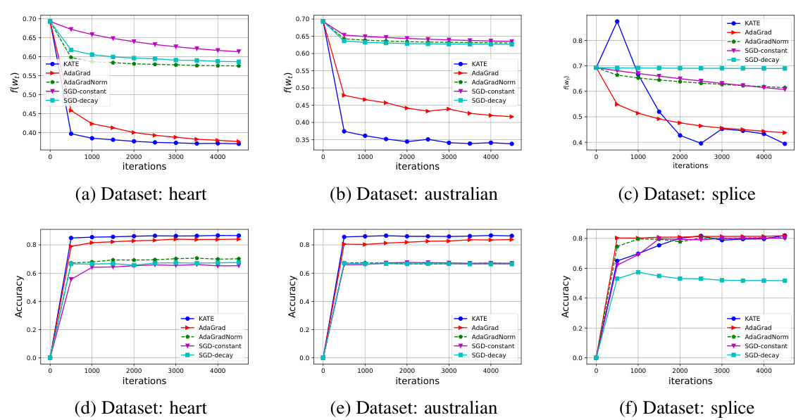
🔼 The figure compares the performance of KATE against four other algorithms (AdaGrad, AdaGradNorm, SGD-decay, and SGD-constant) on three different datasets from LIBSVM (heart, australian, and splice). The plots show both the functional value (loss) and the accuracy over 5000 iterations. This illustrates KATE’s performance in comparison to other methods on real-world datasets.
read the caption
Figure 2: Comparison of KATE with AdaGrad, AdaGradNorm, SGD-decay and SGD-constant on datasets heart, australian, and splice from LIBSVM. Figures 2a, 2b and 2c plot the functional value f(wt), while 2d, 2e and 2f plot the accuracy on y-axis for 5, 000 iterations.

🔼 This figure compares the performance of KATE against AdaGrad, AdaGradNorm, SGD with decay, and SGD with constant step size on a logistic regression task. The x-axis represents different values of Δ, a hyperparameter related to scaling. The y-axis in subfigures (a), (b), and (c) shows the functional value f(wt) at various iteration counts (104, 5 * 104, and 105, respectively). The experiment highlights KATE’s robustness and scale invariance across different initializations.
read the caption
Figure 1: Comparison of KATE with AdaGrad, AdaGradNorm, SGD-decay and SGD-constant for different values of ∆ (on x-axis) for logistic regression model. Figure 1a, 1b and 1c plots the functional value f (wt) (on y-axis) after 104, 5 × 10⁴, and 105 iterations respectively.
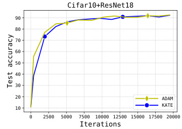
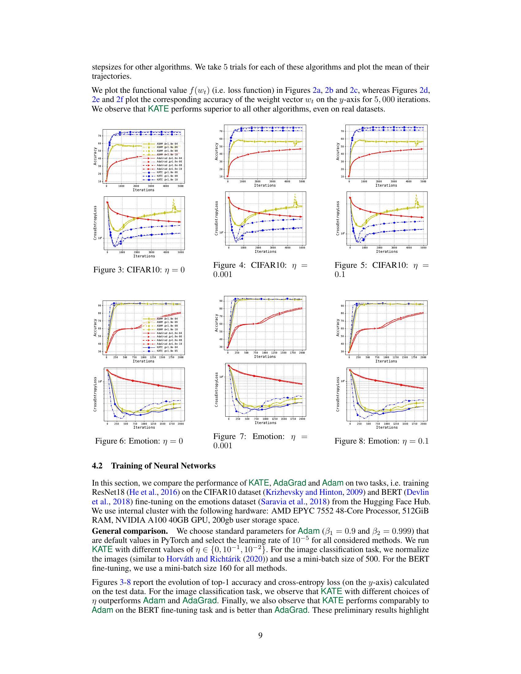
🔼 This figure compares the performance of KATE, AdaGrad and Adam on the task of training ResNet18 on the CIFAR10 dataset. The x-axis represents the number of iterations, and the y-axis shows both the test accuracy and cross-entropy loss. Different learning rates (indicated by different colors and line styles) are used for each algorithm. The figure demonstrates that KATE achieves better performance than AdaGrad and Adam across a range of learning rates.
read the caption
Figure 3: CIFAR10: η = 0

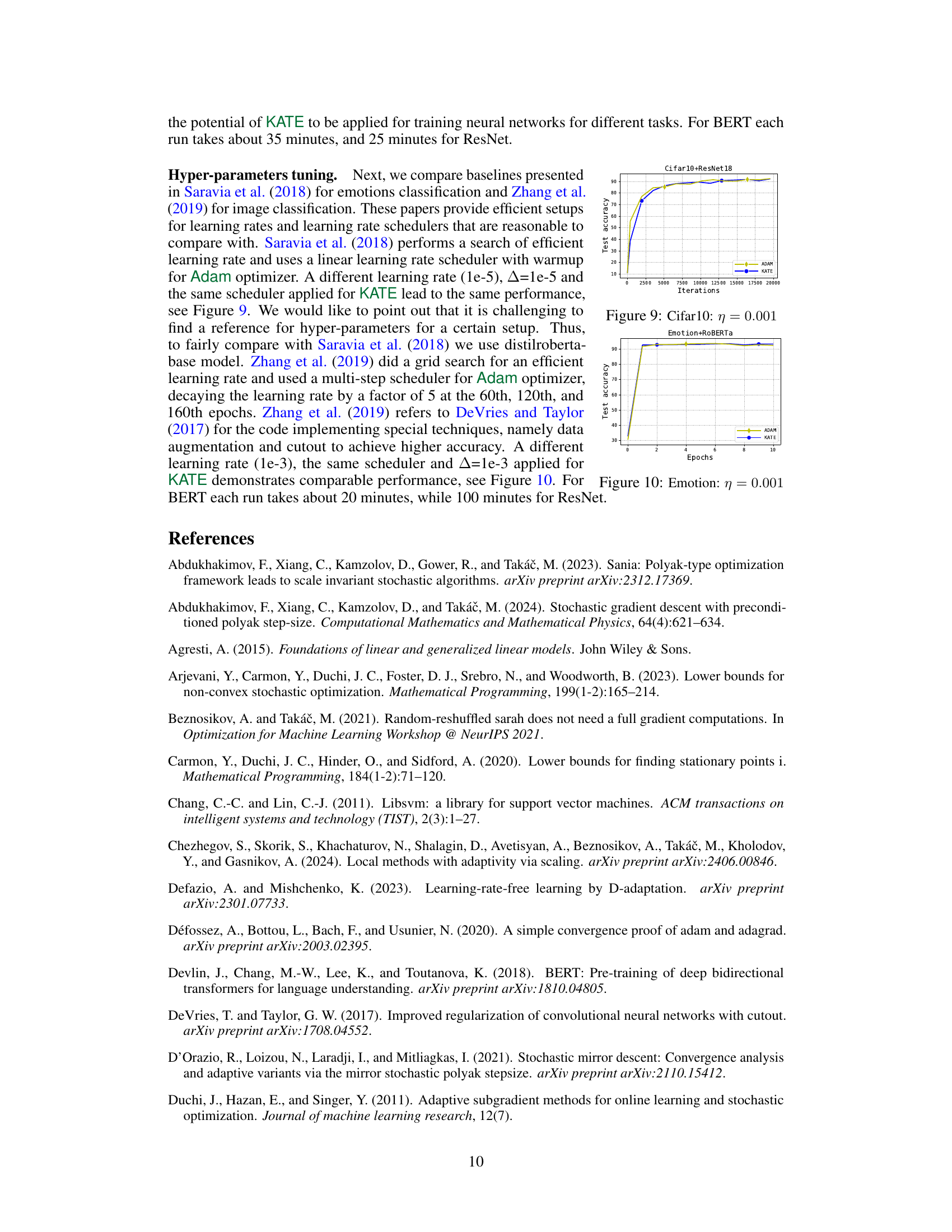
🔼 This figure compares the performance of KATE and Adam optimizers on the emotion classification task using the RoBERTa model. The x-axis represents the number of epochs (training iterations), and the y-axis shows the test accuracy. The plot demonstrates that KATE achieves comparable performance to Adam on this specific task.
read the caption
Figure 10: Emotion: η = 0.001

🔼 This figure compares the performance of KATE against AdaGrad, AdaGradNorm, SGD with decay, and SGD with constant step size on a logistic regression task. The x-axis represents different values of ∆ (a hyperparameter), while the y-axis shows the functional value (loss) after 104, 5 × 10⁴, and 105 iterations (across subfigures (a), (b), and (c), respectively). The results illustrate KATE’s robustness and superior performance across a range of ∆ values, highlighting its adaptability and efficiency.
read the caption
Figure 1: Comparison of KATE with AdaGrad, AdaGradNorm, SGD-decay and SGD-constant for different values of ∆ (on x-axis) for logistic regression model. Figure 1a, 1b and 1c plots the functional value f (wt) (on y-axis) after 104, 5 × 10⁴, and 105 iterations respectively.

🔼 This figure demonstrates the scale invariance of KATE. Subfigures (a) and (b) show that the functional value and accuracy are virtually identical for both scaled and unscaled datasets, supporting the theoretical findings of scale invariance. Subfigure (c) further corroborates this by showing that the gradient norms are also the same for scaled and unscaled data. This indicates the algorithm’s performance is unaffected by data scaling.
read the caption
Figure 11: Comparison of KATE on scaled and un-scaled data. Figures 11a, and 11b plot the functional value f(wt) and accuracy on scaled and unscaled data, respectively. Figure 11c plots ||∇f(wt)||² and ||∇f(wt)||v-2 for unscaled and scaled data respectively.

🔼 This figure compares the performance of the AdaGrad algorithm on scaled and unscaled data. Subfigure (a) shows the functional value f(wt) over iterations for both datasets. Subfigure (b) displays the accuracy achieved on both datasets, and subfigure (c) shows the gradient norms (||∇f(wt)||² and ||∇f(wt)||v-2) for the unscaled and scaled datasets, respectively, to demonstrate the lack of scale invariance of AdaGrad.
read the caption
Figure 12: Comparison of AdaGrad on scaled and un-scaled data. Figures 12a, and 12b plot the functional value f(wt) and accuracy on scaled and unscaled data, respectively. Figure 12c plots ||∇f(wt)||² and ||∇f(wt)||v-2 for unscaled and scaled data respectively.
Full paper#
