TL;DR#
Point cloud assembly, aligning two 3D point clouds, is crucial in various fields but faces challenges like non-overlapping data and sensitivity to initial positions. Traditional correspondence-based methods struggle with these, failing when points don’t directly align. This leads to inaccurate and unreliable alignment, hindering applications in robotics and 3D reconstruction.
This research proposes BITR (SE(3)-bi-equivariant Transformers), a new approach tackling these limitations. BITR uses a transformer network that leverages SE(3)-bi-equivariance, a powerful mathematical property ensuring consistent output even when the inputs are rotated or moved. Theoretically proven and empirically validated, BITR excels in handling non-overlapping point clouds, significantly improving accuracy and stability, which is shown by experiments with diverse datasets.
Key Takeaways#
Why does it matter?#
This paper is crucial for researchers in robotics, computer vision, and machine learning due to its introduction of BITR, a novel and efficient method for point cloud assembly. BITR’s unique SE(3)-bi-equivariance property ensures robustness and accuracy, even with non-overlapping point clouds and varying initial positions. This advancement directly addresses a significant challenge in current 3D data processing, opening doors for improvements in various applications such as robot manipulation and 3D object recognition.
Visual Insights#

🔼 This figure shows two examples of point cloud (PC) assembly, a task where the goal is to find a rigid transformation that aligns one PC to another. The left side displays the input point clouds: (a) shows an example where the point clouds partially overlap, (b) shows an example where they do not overlap. The red point cloud represents the source PC, and the blue represents the reference PC. The right side shows the results of applying the proposed method (BITR) – the red point clouds have been transformed to align with the blue reference point clouds.
read the caption
Figure 1: Two examples of PC assembly. Given a pair of PCs, the proposed method BITR transforms the source PC (red) to align the reference PC (blue). The input PCs may be overlapped (a) or non-overlapped (b).

🔼 This table presents a comparison of the performance of different methods on the 2-fragment WineBottle dataset, specifically focusing on the rotation and translation errors. The results demonstrate that BITR outperforms other methods (DGL, NSM, LEV) achieving the lowest rotation error and a translation error comparable to the best performing method, DGL.
read the caption
Table 1: Reassembly results on 2-fragment WineBottle. We report the mean and std of the error of BITR.
In-depth insights#
SE(3)-Equivariance in Assembly#
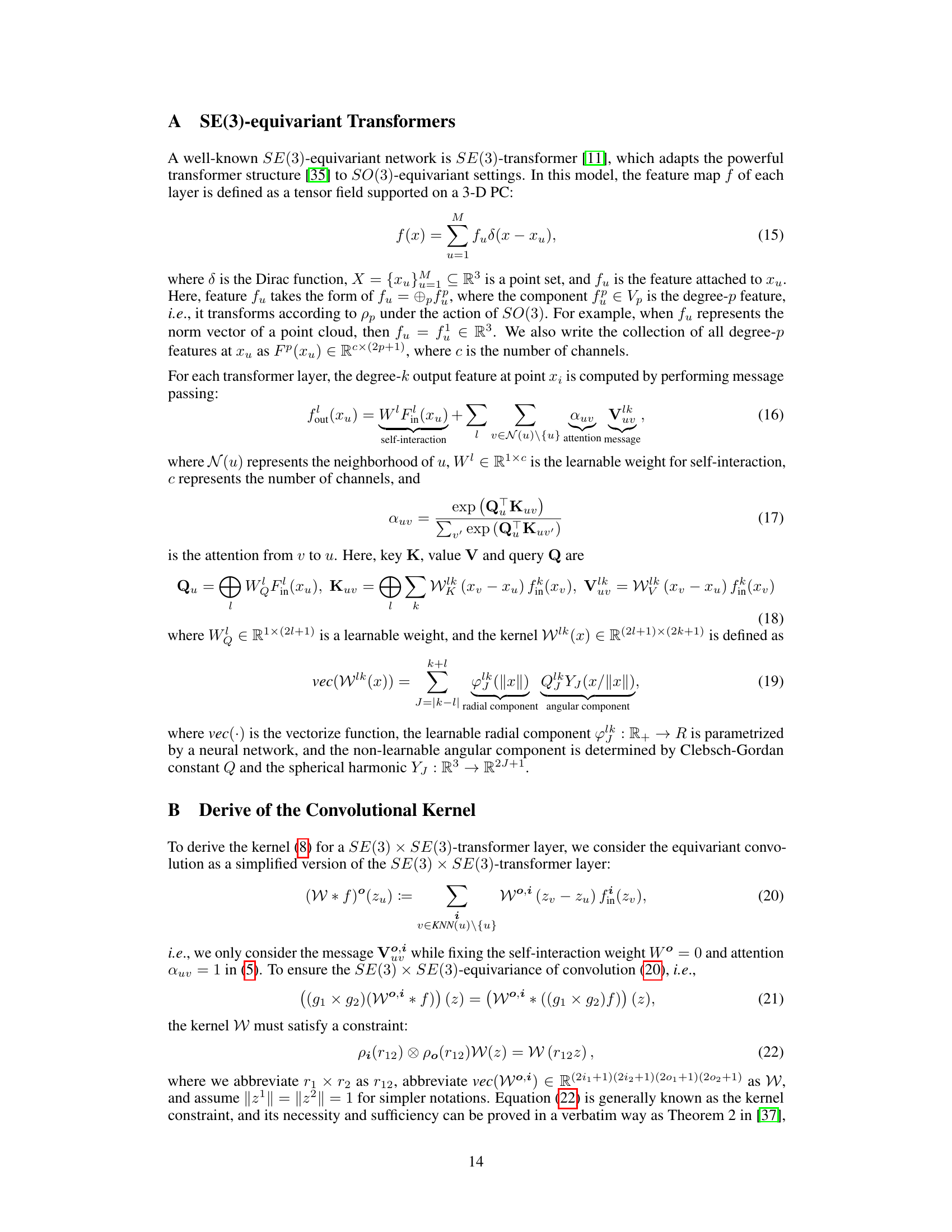
The concept of SE(3)-equivariance applied to assembly tasks offers a powerful framework for developing robust and accurate algorithms. SE(3) represents the group of rigid transformations in 3D space (rotations and translations). An SE(3)-equivariant assembly method would ensure that if the input point clouds are transformed rigidly, the output (e.g., the estimated transformation aligning the clouds) undergoes the same transformation. This is crucial because it guarantees that the algorithm’s performance is not affected by arbitrary initial positions or orientations of the parts. Equivariance simplifies learning by reducing the complexity of the problem, as the algorithm only needs to learn the relationship between the shapes themselves rather than needing to handle all possible poses. The method inherently addresses challenges of non-overlapping point clouds, a common issue in real-world assembly. By explicitly incorporating SE(3)-equivariance, the network’s inherent understanding of 3D geometry is enhanced, leading to better generalization and robustness. However, achieving true SE(3)-equivariance can be computationally expensive; therefore, finding efficient implementations is key for practical applications. Future research should focus on this efficiency, as well as the theoretical properties of the approach and its limitations.
BITR Architecture#
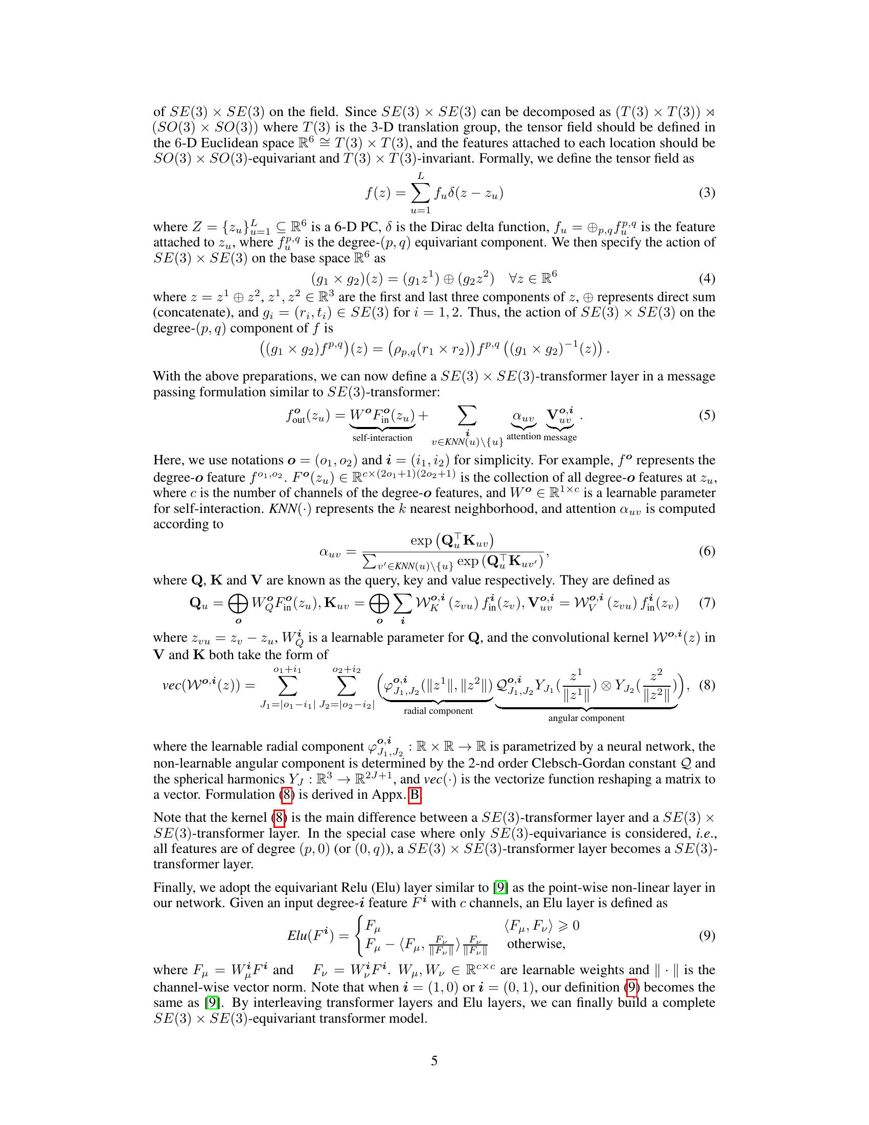
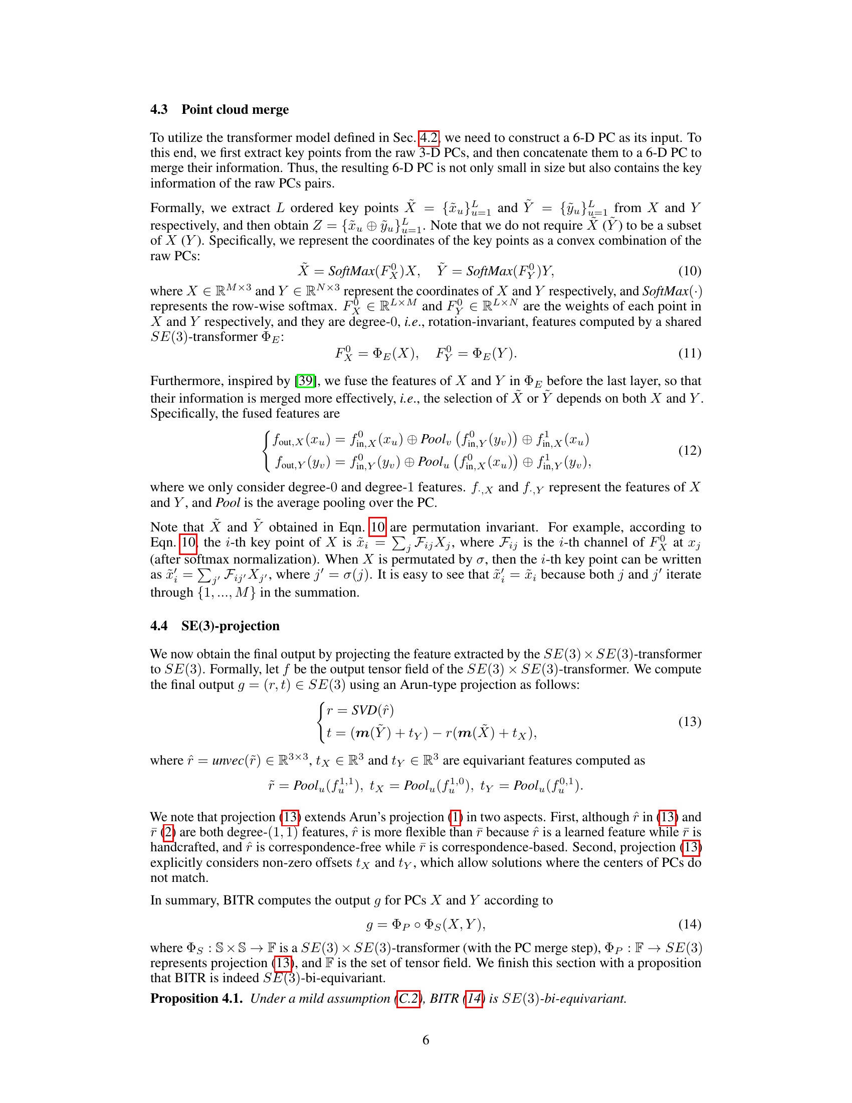
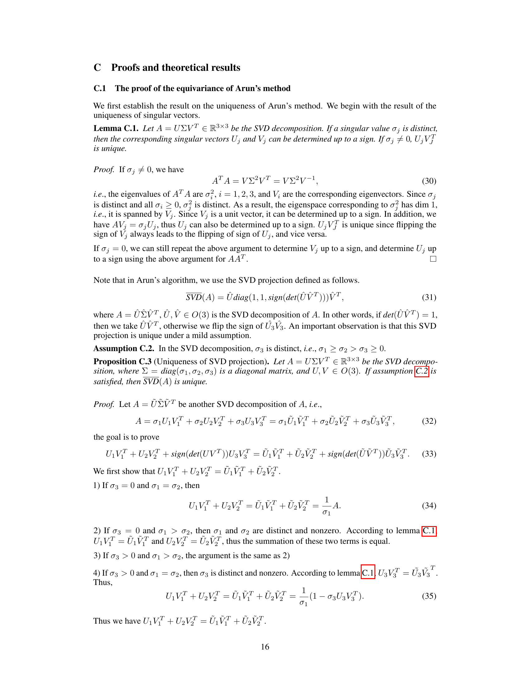
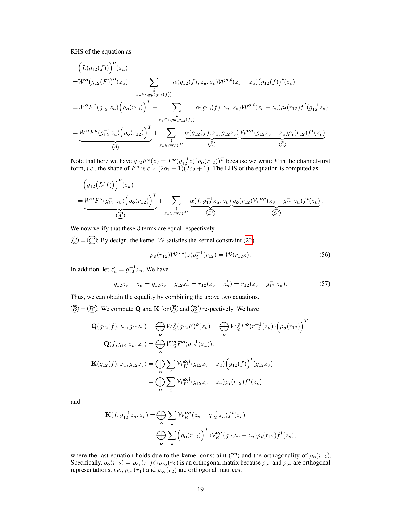
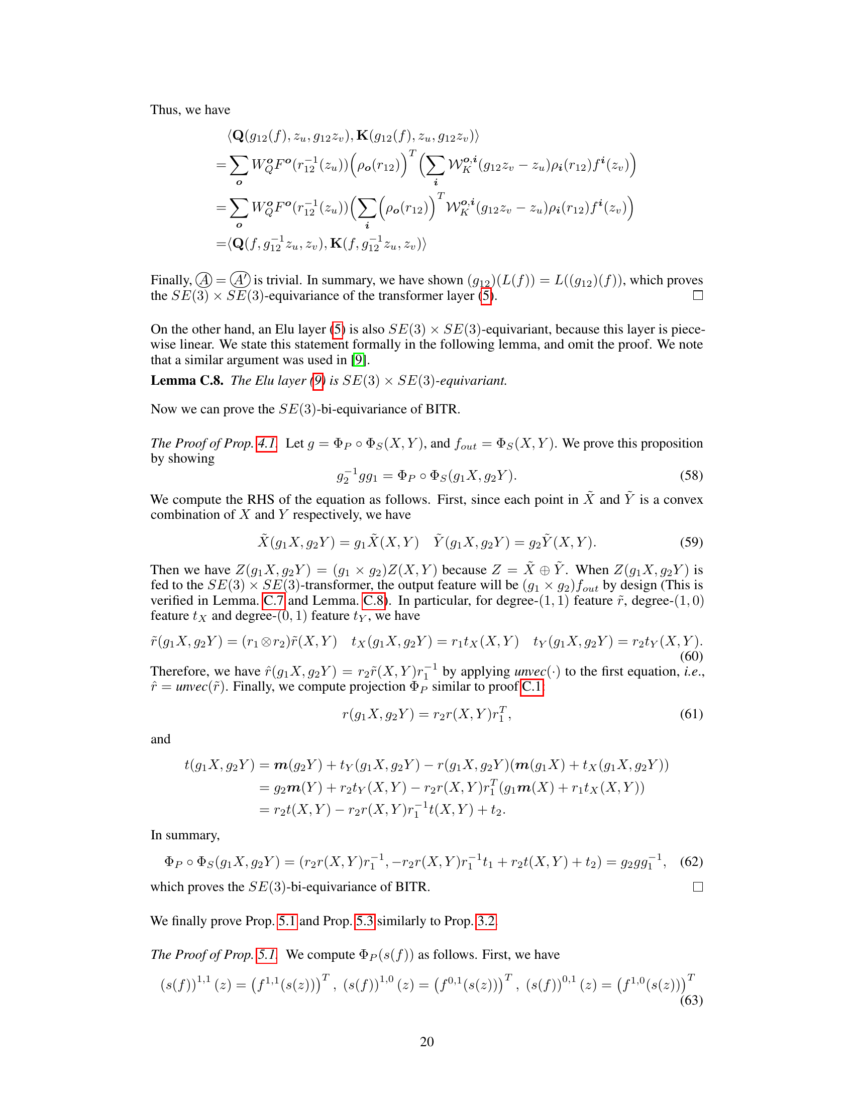
The BITR architecture is a novel approach to point cloud assembly, combining SE(3)-bi-equivariant transformers with a point cloud merge strategy. This design directly addresses the challenges of non-overlapping point clouds and initial pose variation. The key innovation lies in its use of an SE(3) × SE(3)-transformer, which extracts features exhibiting both rotational equivariance and translational invariance. This allows BITR to handle arbitrary initial positions and non-overlapped point clouds which are typically problematic for correspondence-based methods. The subsequent projection into SE(3) leverages Arun’s method for efficient rigid transformation estimation. Furthermore, the integration of swap and scale equivariances enhances BITR’s robustness to variations in input scaling and order, leading to improved stability and performance. The architecture is end-to-end trainable, eliminating the need for explicit correspondence estimation, making it a significant advancement in the field.
Equivariance Properties#
Equivariance, a crucial concept in this research, ensures that when input data undergoes a transformation (like rotation or scaling), the output predictably transforms in a corresponding manner. This symmetry property is particularly valuable for tasks involving point cloud assembly, as it guarantees consistent performance regardless of the initial orientation or scale of the objects. The paper thoroughly investigates different types of equivariance, including SE(3)-bi-equivariance, scale-equivariance, and swap-equivariance. SE(3)-bi-equivariance, by handling rigid transformations of both input point clouds, is key to robustness. The theoretical analysis rigorously demonstrates how these properties are incorporated into the proposed model, ultimately leading to a more stable and reliable system. The theoretical proofs provide strong mathematical grounding for the observed empirical results, highlighting the benefits of leveraging the equivariance principles. Moreover, this work demonstrates that incorporating these equivariance properties is not merely a theoretical exercise, but directly impacts the practical performance of the point cloud assembly task, exhibiting superior robustness against various perturbations.
Assembly Experiments#
In a hypothetical research paper section titled ‘Assembly Experiments,’ one would expect a rigorous evaluation of a proposed point cloud assembly method. This would involve a multifaceted approach, likely including experiments on synthetic datasets to control variables and assess performance under various conditions (e.g., varying degrees of overlap, noise levels, object scales, and initial poses). Further experiments on real-world datasets are crucial for demonstrating the method’s practical applicability and robustness. A comparison against existing state-of-the-art methods is essential, using standardized metrics like rotation and translation error to quantify performance. The results should be presented clearly, with statistical significance analysis, including error bars and confidence intervals, ensuring reproducibility. It would be valuable to see an ablation study removing key components to understand their individual contributions. Finally, a discussion of the method’s limitations and potential future work would conclude this section, focusing on challenges like computational efficiency and the handling of incomplete or noisy data.
Future Research#
The paper’s “Future Research” section hints at several promising avenues. Improving computational efficiency is paramount, especially addressing the independent computation of convolutional kernels. Exploring acceleration techniques like those used in SO(3)-equivariant networks is a key area. Addressing the limitations in handling symmetric point clouds is crucial, possibly by transitioning to a generative model that assigns likelihoods to multiple possible alignments. Extending the model to handle multi-point cloud assembly is another important goal. Finally, investigating the use of U-BITR in self-supervised 3D shape retrieval tasks could provide valuable insights and demonstrate real-world applications.
More visual insights#
More on figures

🔼 This figure shows two examples of point cloud (PC) assembly, a task where the goal is to find the rigid transformation that aligns one PC (the source) to another (the reference). The figure illustrates two scenarios: (a) where the source and reference PCs overlap, and (b) where they do not. In both cases, the proposed method, BITR, transforms the red (source) PC to match the blue (reference) PC.
read the caption
Figure 1: Two examples of PC assembly. Given a pair of PCs, the proposed method BITR transforms the source PC (red) to align the reference PC (blue). The input PCs may be overlapped (a) or non-overlapped (b).
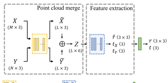
🔼 This figure shows the architecture of the proposed method, SE(3)-bi-equivariant transformer (BITR). It illustrates the two main steps: 1) Point cloud merge, where the input point clouds X and Y are merged into a 6D point cloud Z by extracting and concatenating keypoints. 2) Feature extraction, where the 6D point cloud Z is passed through a SE(3) x SE(3)-transformer to extract equivariant features (r̂, tx, ty). Finally, these features are projected into the SE(3) group to obtain the final output, which is the rigid transformation.
read the caption
Figure 2: An overview of BITR. The input 3-D PCs X and Y are first merged into a 6-D PC Z by concatenating the extracted key points X and Y. Then, Z is fed into a SE(3) × SE(3)-transformer to obtain equivariant features î, tx and ty. These features are finally projected to SE(3) as the output.

🔼 This figure shows four point cloud assembly results from the BITR model. The first image shows the original input point clouds (source and reference). The subsequent three images show results from the same input point clouds but with different transformations: swapped (source and reference PCs are exchanged), rigidly perturbed (source and reference are rotated and translated), and scaled (source and reference PCs are scaled). The consistency of the results across these transformations demonstrates the model’s robustness to changes in input orientation, position, and scale.
read the caption
Figure 3: The results of BITR on a test example (a), and the swapped (b), scaled (d) and rigidly perturbed (c) inputs. The red, yellow and blue colors represent the source, transformed source and reference PCs respectively.

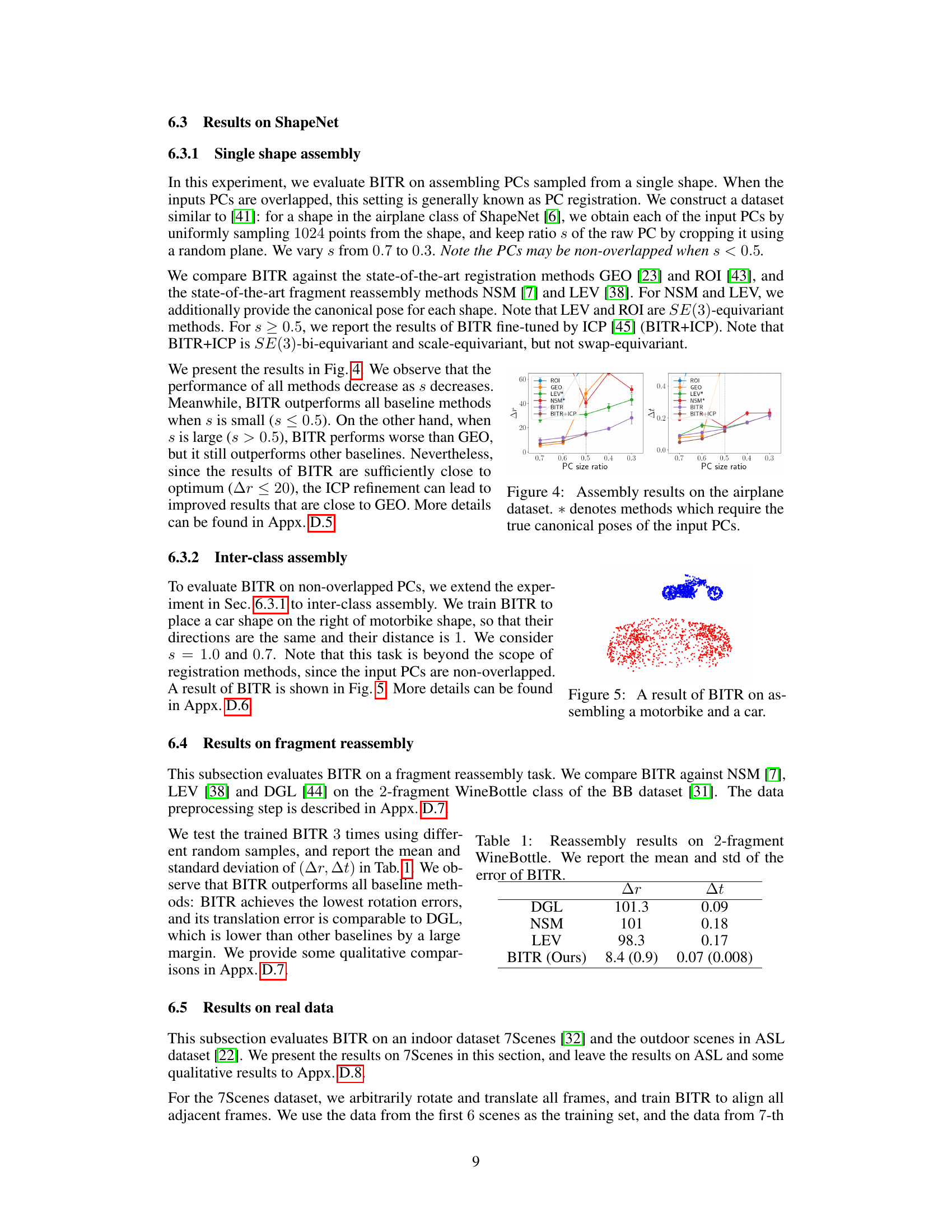
🔼 This figure shows the performance comparison of different methods for the airplane dataset. The x-axis represents the PC size ratio (the percentage of the raw PC kept by cropping). The y-axis on the left shows the rotation error (∆r), and the y-axis on the right shows the translation error (∆t). The methods compared include GEO, ROI, NSM, LEV, BITR, and BITR+ICP. The asterisk (*) indicates that the methods require the true canonical poses of the input PCs. The results indicate that BITR outperforms other methods when the PC size ratio is small (less overlap), and its performance is close to the best methods when the PC size ratio is large (more overlap), especially with ICP refinement.
read the caption
Figure 4: Assembly results on the airplane dataset. * denotes methods which require the true canonical poses of the input PCs.

🔼 This figure shows an example of the BITR method assembling two point clouds representing a motorbike and a car. The goal is to find the rigid transformation that aligns the source point cloud (the car) to the reference point cloud (the motorbike). This illustrates the capability of BITR to handle non-overlapped point clouds, a significant challenge in point cloud assembly.
read the caption
Figure 5: A result of BITR on assembling a motorbike and a car.

🔼 This figure shows two examples of the results from applying the BITR model to the bowl-placing task. The left panels show the initial configurations of the bowl (red) and plate (green). The right panels show the results of applying the BITR algorithm. The first example demonstrates a successful placement where the bowl is correctly positioned on the plate. The second example shows a failure case where the bowl is incorrectly positioned, resulting in a collision. The gray points in the figures represent the environment.
read the caption
Figure 6: The results of BITR on bowl-placing. We present the input PCs (left panel) and the assembled results (right panel). BITR can generally place the bowl (red) on the plate (green) (a), but it sometimes produces unrealistic results where collision exists (b).

🔼 This figure shows the results of applying BITR to a test example and its variations. The first image (a) displays the original result, while (b), (c), and (d) show results for swapped, rigidly perturbed, and scaled inputs respectively. The consistency of the results across these different scenarios visually demonstrates the method’s robustness to variations in input data and its SE(3)-bi-equivariance, swap-equivariance and scale-equivariance.
read the caption
Figure 3: The results of BITR on a test example (a), and the swapped (b), scaled (d) and rigidly perturbed (c) inputs. The red, yellow and blue colors represent the source, transformed source and reference PCs respectively.

🔼 This figure shows the training curves of the proposed BITR model on the airplane dataset. The curves display the loss function, rotation error (Δr), and translation error (Δt) over 10000 training epochs. The metrics are calculated using the validation set to monitor the model’s performance and prevent overfitting. The curves show a general downward trend, indicating that the model is learning and improving its accuracy throughout the training process. The slight fluctuations in the curves may represent the model’s progress in learning complex features or might be due to the stochastic nature of the training process.
read the caption
Figure 8: The training process of BITR on the airplane dataset with s = 0.4. All metrics are measured on the validation set.

🔼 This figure shows four examples of point cloud registration using the proposed BITR method. Each subfigure shows the input point clouds (in light colors) and the 32 key points (in dark colors). The goal is to align the red point cloud (source) to the blue point cloud (reference). Different values of the size ratio s (0.7, 0.5, 0.4, and 0.3) are used in different subfigures. These different size ratios demonstrate that the method can handle various degrees of overlap between the point clouds.
read the caption
Figure 9: The PC registration results of BITR on the airplane dataset. The input PCs are represented using light colors, and the learned key points are represented using dark and large points.
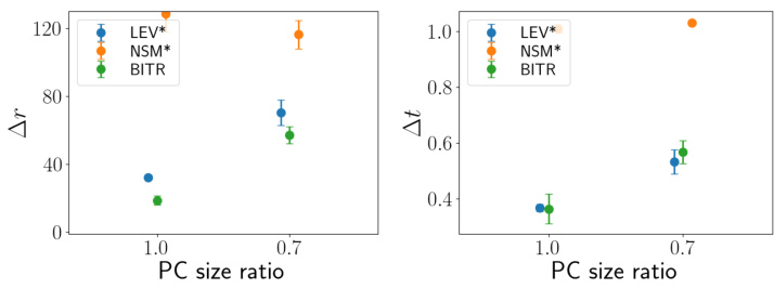
🔼 This figure shows the performance comparison of different methods for the airplane dataset in terms of PC size ratio. The x-axis represents the PC size ratio (s), which varies from 0.3 to 0.7. The y-axis represents the rotation error (∆r). The figure shows that BITR outperforms all baseline methods when s is small (s ≤ 0.5). When s is large (s > 0.5), BITR performs worse than GEO, but still outperforms other baselines. However, since BITR results are sufficiently close to optimum (∆r ≤ 20), ICP refinement can lead to improved results that are close to GEO. The methods marked with ‘*’ require the true canonical poses of the input PCs.
read the caption
Figure 4: Assembly results on the airplane dataset. * denotes methods which require the true canonical poses of the input PCs.

🔼 This figure compares the results of reassembling wine bottle fragments using four different methods: DGL, NSM, LEV, and the proposed BITR method. Each method is shown assembling the same fragments, allowing a visual comparison of their performance. The results highlight BITR’s superior performance in this task.
read the caption
Figure 11: Results of reassembling wine bottle fragments. We compare the proposed BITR with DGL [44], NSM [7] and LEV [38]. Zoom in to see the details.

🔼 This figure shows two examples of point cloud (PC) assembly using the proposed method, BITR. In (a), two overlapped PCs representing the same object are shown before and after alignment. In (b), two non-overlapped PCs are shown, also before and after alignment with BITR. The red PC represents the source PC that is transformed using BITR to align it with the blue reference PC.
read the caption
Figure 1: Two examples of PC assembly. Given a pair of PCs, the proposed method BITR transforms the source PC (red) to align the reference PC (blue). The input PCs may be overlapped (a) or non-overlapped (b).
🔼 This figure shows the results of the proposed method, BITR, on a test example and three variations of the input. (a) shows the original test example, (b) shows the result when the source and target point clouds are swapped, (c) shows the result when the inputs are randomly rotated and translated, and (d) shows the result when the inputs are scaled. The consistent results demonstrate the method’s robustness to different input configurations and its equivariance properties.
read the caption
Figure 3: The results of BITR on a test example (a), and the swapped (b), scaled (d) and rigidly perturbed (c) inputs. The red, yellow and blue colors represent the source, transformed source and reference PCs respectively.
More on tables
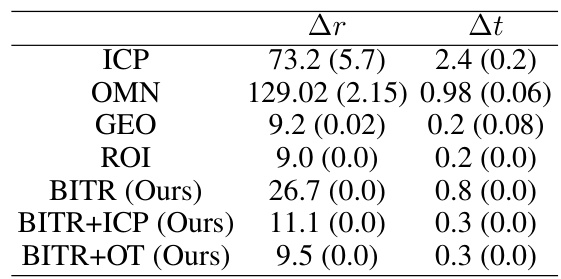
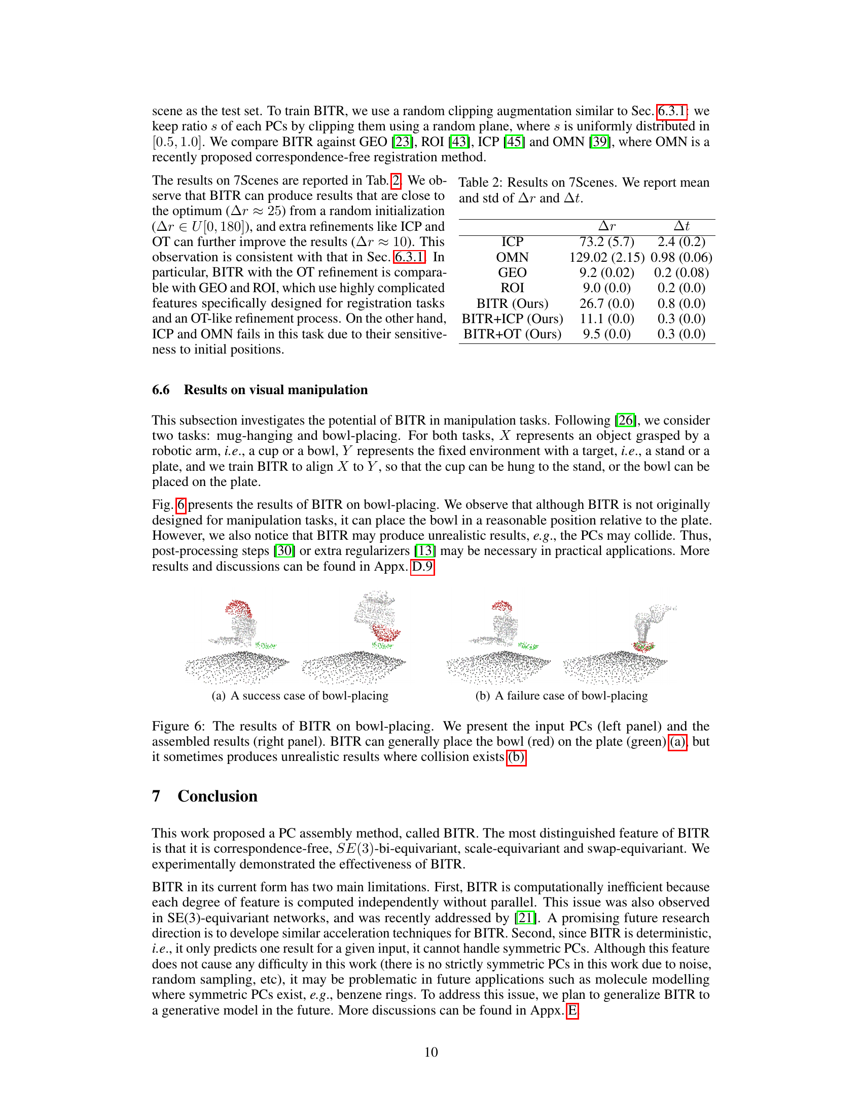
🔼 This table presents the quantitative results of different methods on the 7Scenes dataset. It shows the mean and standard deviation of the rotation error (Δr) and translation error (Δt) for various methods, including ICP, OMN, GEO, ROI, and the proposed BITR method, with and without refinement using ICP and OT.
read the caption
Table 2: Results on 7Scenes. We report mean and std of Δr and Δt.

🔼 This table presents the quantitative results to verify the SE(3)-bi-equivariance, swap-equivariance and scale-equivariance of BITR. The values represent the Frobenius norm of the difference between the expected transformation and the BITR’s output for various perturbations. Very small values close to numerical precision indicate strong support for the claimed equivariances.
read the caption
Table 3: Verification of the equivariance of BITR.

🔼 This ablation study demonstrates the impact of removing swap or scale equivariance from the BITR model. The results show the mean and standard deviation of the rotation error (Ar) for the original, rigidly perturbed, swapped, and scaled test cases. Removing swap equivariance significantly affects the results when the input point clouds are swapped, and removing scale equivariance substantially impacts the results when the input point clouds are scaled.
read the caption
Table 4: Ablation study of scale and swap equivariances. We report mean and std of Ar

🔼 This table presents the results of the untrained BITR (U-BITR) method for the complete matching problem under different conditions. The conditions tested include an ideal scenario where X and Y are identical, scenarios with resampling, added Gaussian noise, and a reduction in the size of X and Y via cropping. The results are evaluated using the rotation error (Δr) and translation error (Δt), showing the method’s performance in various noisy and incomplete data settings.
read the caption
Table 5: Results of complete matching using U-BITR.
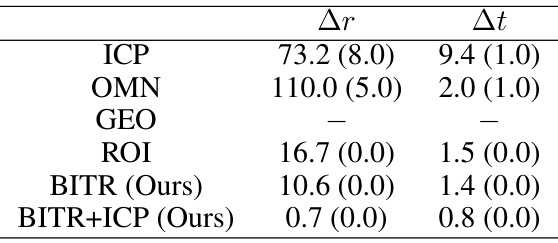
🔼 This table presents the results of the experiment conducted on the outdoor scenes of ASL dataset. The mean and standard deviation of rotation error (Ar) and translation error (At) are reported for different methods: ICP, OMN, GEO, ROI, BITR, and BITR+ICP. The results show the performance of BITR in comparison to other methods for the task of aligning adjacent frames in outdoor scenes.
read the caption
Table 6: Results on the outdoor scenes of ASL. We report mean and std of Ar and At.
Full paper#


