↗ OpenReview ↗ NeurIPS Homepage ↗ Chat
TL;DR#
Many real-world optimization problems involve constraints on the order of evaluations, limiting the flexibility of traditional Bayesian Optimization (BayesOpt) methods. These constraints often arise from physical limitations or sequential dependencies inherent in the system being optimized. Existing BayesOpt techniques struggle in these scenarios because they don’t account for these transition constraints, resulting in suboptimal solutions.
This paper tackles this limitation by integrating BayesOpt with the framework of Markov Decision Processes (MDPs). The authors propose a novel utility function based on maximum identification via hypothesis testing and iteratively solve a tractable linearization using reinforcement learning to plan ahead for the entire horizon. The resulting policy is potentially non-Markovian, adapting to the history of previous decisions and system dynamics. The approach is validated on various synthetic and real-world examples, demonstrating its ability to handle complex transition constraints effectively and improve the efficiency of optimization.
Key Takeaways#
Why does it matter?#
This paper is crucial for researchers in Bayesian Optimization and Reinforcement Learning, particularly those tackling real-world problems with transition constraints. It presents a novel framework for planning ahead, enabling the optimization of complex systems where sequential decisions are limited by inherent dynamics. This research offers significant advancements in tackling challenges across various scientific domains, paving the way for more effective strategies in scenarios previously difficult to handle.
Visual Insights#

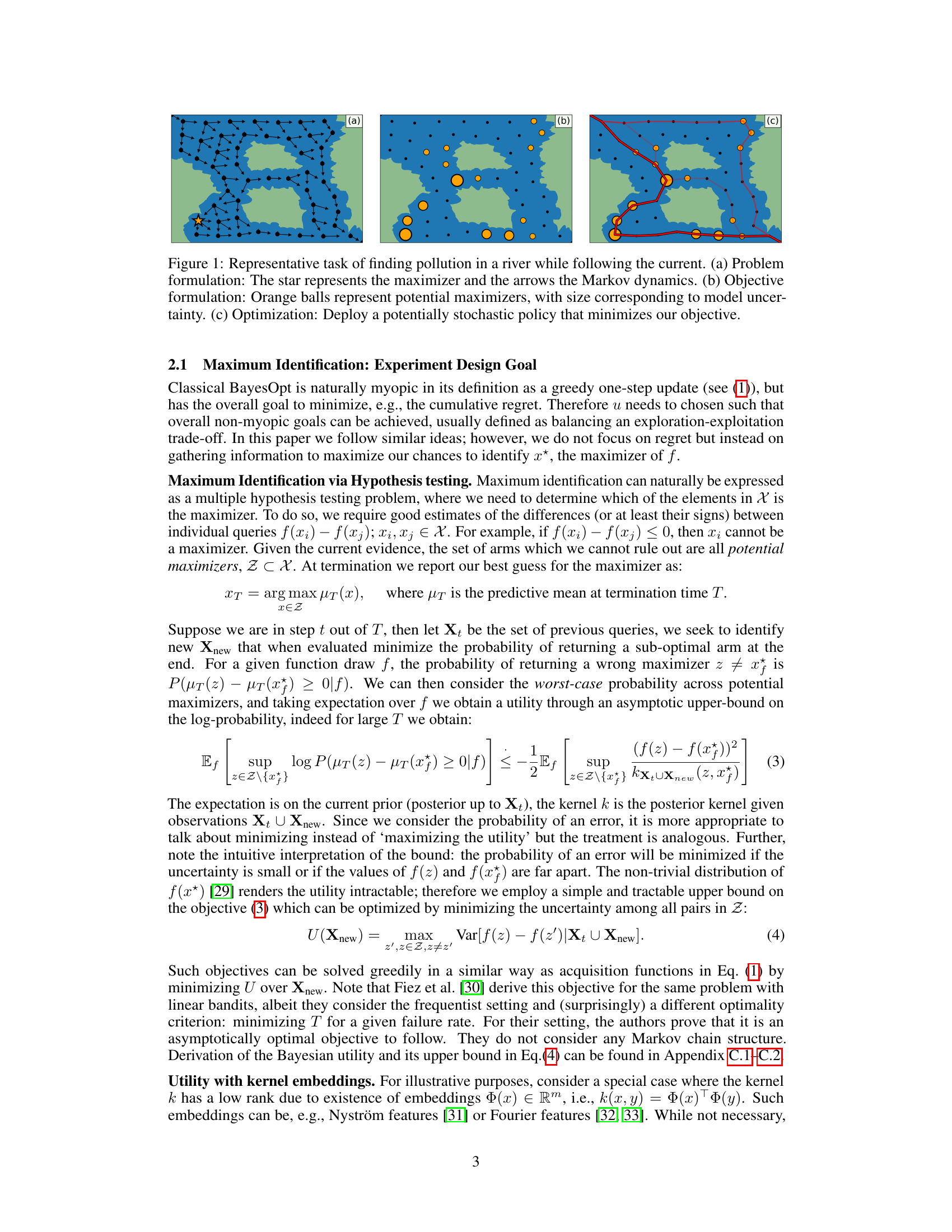
This figure illustrates an application of the proposed method to environmental monitoring. Panel (a) shows the problem setup, where the goal is to find the source of pollution (star) while respecting constraints on movement (arrows). Panel (b) illustrates how the uncertainty in the pollution levels is modeled, with larger orange circles representing higher uncertainty. Panel (c) demonstrates how a policy can be created to optimize exploration and minimize the uncertainty.

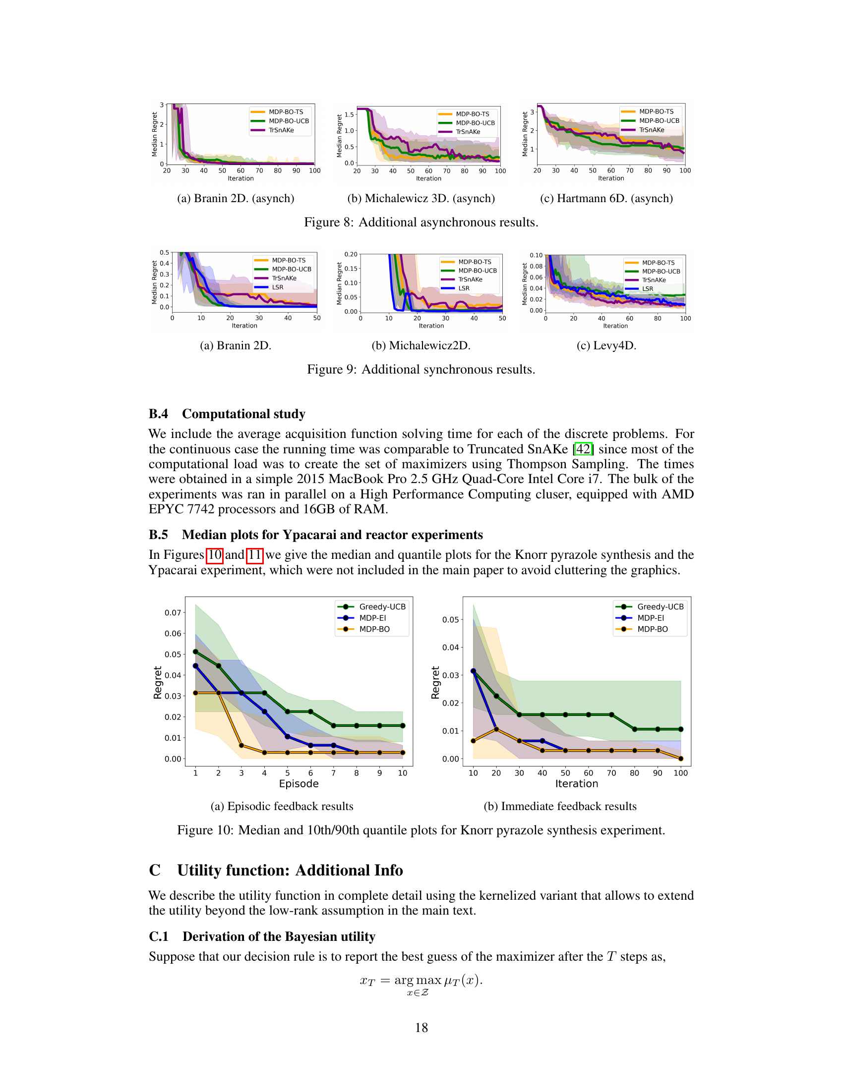
This table presents the computational efficiency of the proposed method by reporting the average solving time of the acquisition function for three real-world benchmarks. The size of the state space, the maximum number of actions possible from each state, and the planning horizon are also provided for context.
In-depth insights#
MDP-BayesOpt Fusion#
MDP-BayesOpt fusion presents a powerful paradigm shift in Bayesian Optimization (BO) by addressing its limitations in scenarios with sequential dependencies and constraints. Traditional BO assumes independent function evaluations, which is unrealistic for many real-world problems where the next evaluation point depends on the previous ones, such as in robotic control or materials science. By integrating Markov Decision Processes (MDPs), the framework explicitly models these dynamics, enabling proactive planning over the entire optimization horizon. This planning aspect is crucial because it allows for a principled method to handle constraints and leverage the history of evaluations. The key to success is in defining a utility function that accounts for both exploration and exploitation while considering the MDP’s transition probabilities. Reinforcement Learning (RL) techniques, such as dynamic programming or approximate dynamic programming, are employed to find optimal policies. This approach results in potentially non-Markovian policies that are history-dependent and superior to purely myopic BO strategies.
Transition Constraints#
The concept of ‘Transition Constraints’ in the context of Bayesian Optimization (BO) signifies the limitations imposed on the sequential exploration of the search space. Unlike traditional BO, where any point can be evaluated next, transition constraints dictate that the next evaluation depends on the current state, thereby introducing a sequential decision-making element. This constraint arises in various real-world applications where there are physical or logical restrictions in moving from one state to another. These constraints can be deterministic, such as limitations on the rate of change of variables, or stochastic, involving probabilistic transitions. The presence of these constraints necessitates a more sophisticated optimization strategy, extending beyond the myopic approach of classical BO. Addressing transition constraints involves incorporating a planning mechanism, commonly by modeling the problem as a Markov Decision Process (MDP). This enables the development of policies that optimize the exploration trajectory, taking into account future consequences of the current action. The challenge then becomes to efficiently and tractably solve the resulting MDP, often through approximate methods, to derive a potentially history-dependent and non-Markovian policy that can navigate the transition constraints effectively.
Planning via MDPs#
The heading ‘Planning via MDPs’ suggests a methodology using Markov Decision Processes (MDPs) to solve planning problems within a given research paper. MDPs are a powerful framework for modeling sequential decision-making under uncertainty, where an agent interacts with an environment by taking actions and receiving rewards. The paper likely demonstrates how the structure of MDPs allows for the explicit incorporation of transition constraints, which are limitations on the allowable state transitions in many real-world scenarios. This is crucial because these constraints often restrict an agent’s choices, necessitating a planning approach that considers future consequences. The use of MDPs probably involves formulating the problem as an optimization process where the objective function is a measure of the desired outcome, such as maximizing reward or minimizing cost. The optimal solution likely involves finding a policy – a mapping from states to actions – that dictates the agent’s behavior at each step. The solution to this problem would likely involve reinforcement learning or dynamic programming techniques to obtain the optimal policy. The paper likely showcases an application where planning under transition constraints is essential and proves the effectiveness of the MDP-based approach in solving such problems.
Tractable Utility#
The concept of “Tractable Utility” in the context of Bayesian Optimization, especially when dealing with transition constraints, is crucial. A tractable utility function is one that can be efficiently optimized, which is vital for the success of any Bayesian Optimization algorithm. The key challenge is balancing the need for a utility function that accurately reflects the value of potential search points against the computational cost of optimizing it. In scenarios with transition constraints, where the search space is not fully explorable at each step, the acquisition function must capture this limitation. A tractable utility is critical for scalability and practical applicability. The complexity arises from the sequential nature of the decision-making process, making the usual direct optimization approaches computationally prohibitive. Therefore, developing approaches for tractable utility functions that incorporate these constraints, such as using linearizations, approximations, or alternative optimization techniques like Frank-Wolfe, becomes essential for effective optimization in this domain. Strategies that balance accuracy, computational efficiency, and consideration of transition constraints are key elements in the design of tractable utility functions that enable practical implementation of transition constrained Bayesian optimization.
Future Extensions#
Future work could explore several promising avenues. Extending the framework to handle more general transition dynamics beyond simple Markov chains is crucial for broader applicability. This might involve incorporating continuous state-action spaces or non-Markovian transitions. Investigating alternative acquisition functions beyond maximum identification, such as regret minimization or other utility functions tailored to specific applications, would offer additional flexibility. Developing efficient algorithms for continuous state and action spaces is vital. While the paper presents approaches to this, further improvements in scalability and computational efficiency are desirable. Thorough investigation of different kernel choices and their impact on performance is also warranted. Finally, a deeper theoretical analysis to provide stronger guarantees on convergence rates and sample complexity would enhance the paper’s contribution.
More visual insights#
More on figures

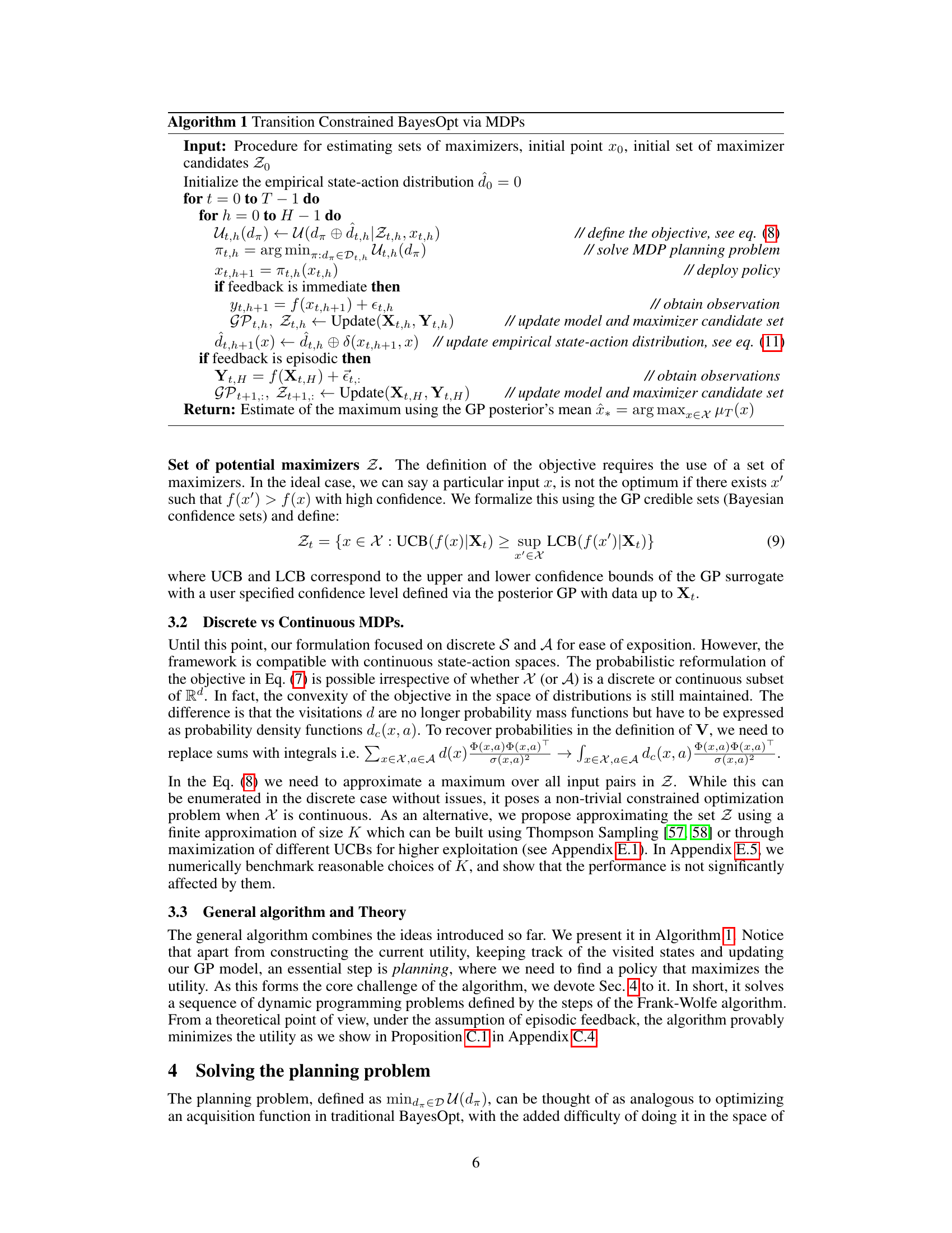
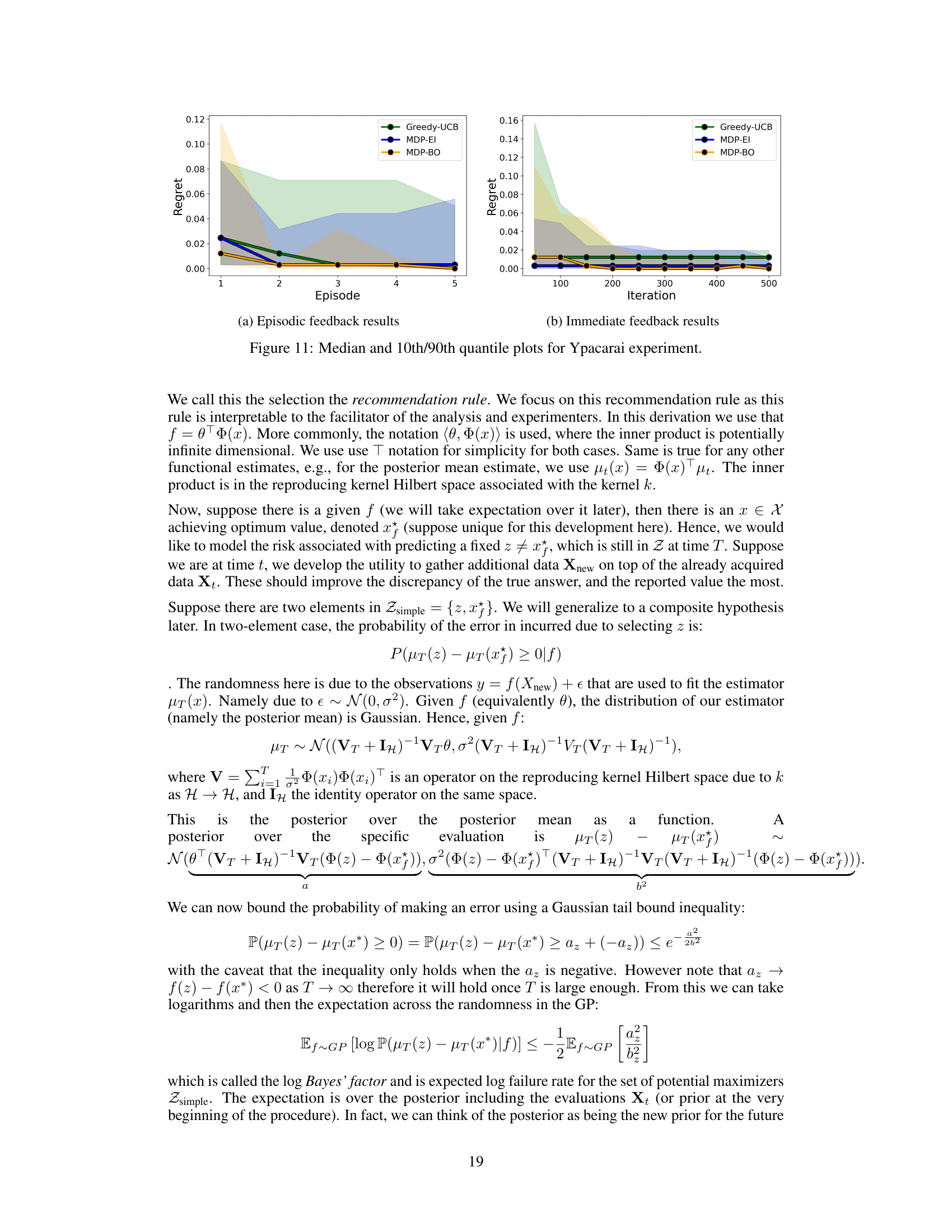
This figure displays the results of the Knorr pyrazole synthesis experiment. The left side shows quantitative results using line plots for best prediction regret and bar charts for the percentage of runs correctly identifying the best arm per episode. The right side shows ten different paths generated by the algorithm, plotted over contours of the underlying black-box function. The paths illustrate how the algorithm navigates the search space while adhering to the specified transition constraints (non-decreasing residence time). The figure highlights the algorithm’s ability to identify the true maximizer while respecting constraints.

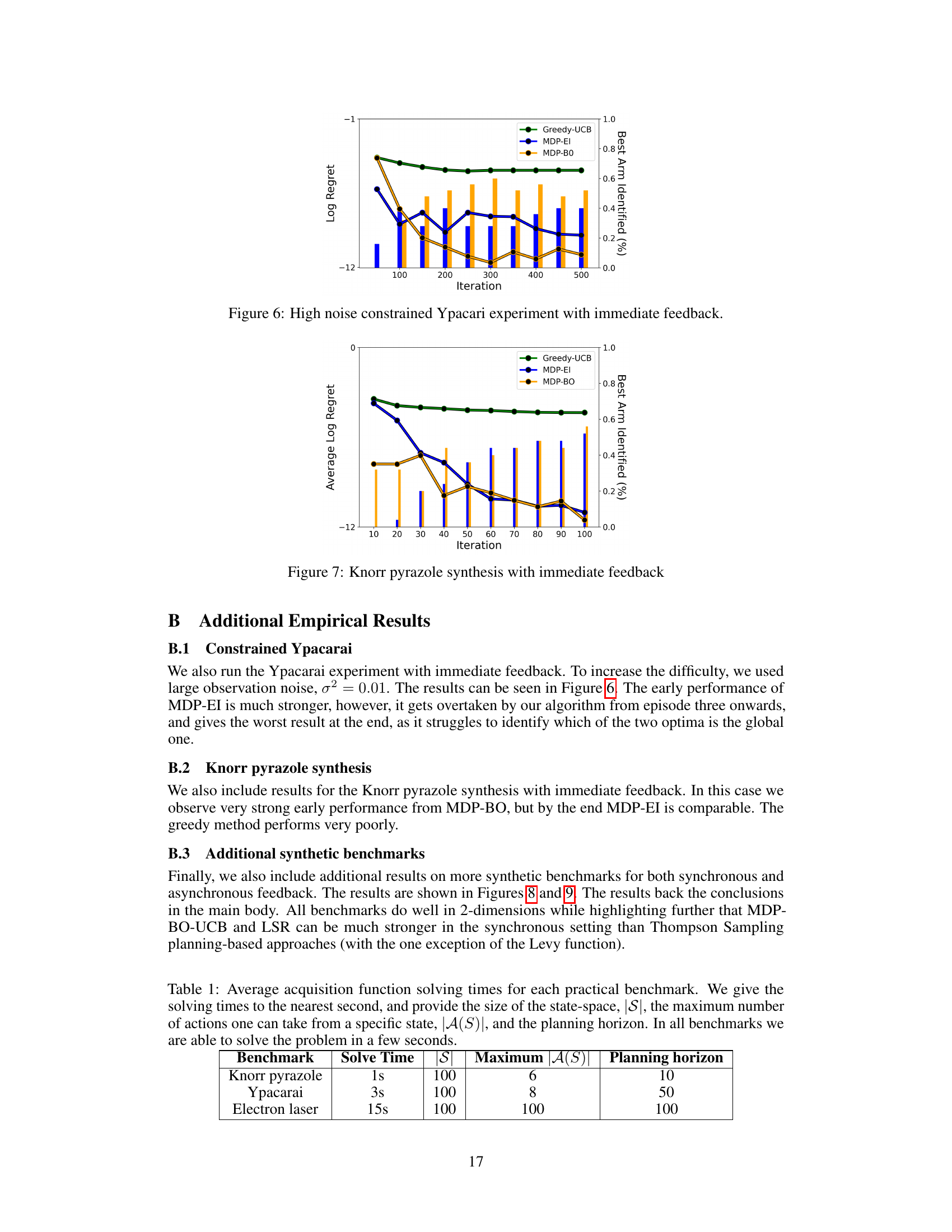
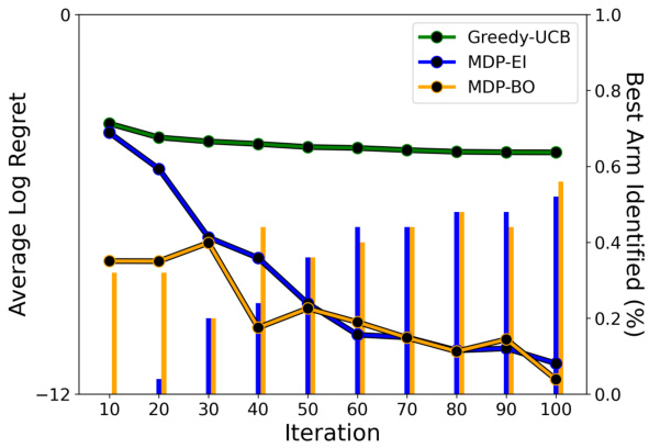
The figure shows the results of the high noise constrained Ypacarai experiment with immediate feedback. The lines represent the average regret, and the bars show the percentage of runs that correctly identified the best arm at the end of each episode. Three different Bayesian Optimization methods are compared: Greedy-UCB, MDP-EI, and MDP-BO. The graph illustrates the performance of each method over multiple episodes, demonstrating MDP-BO’s superior performance in this challenging scenario.

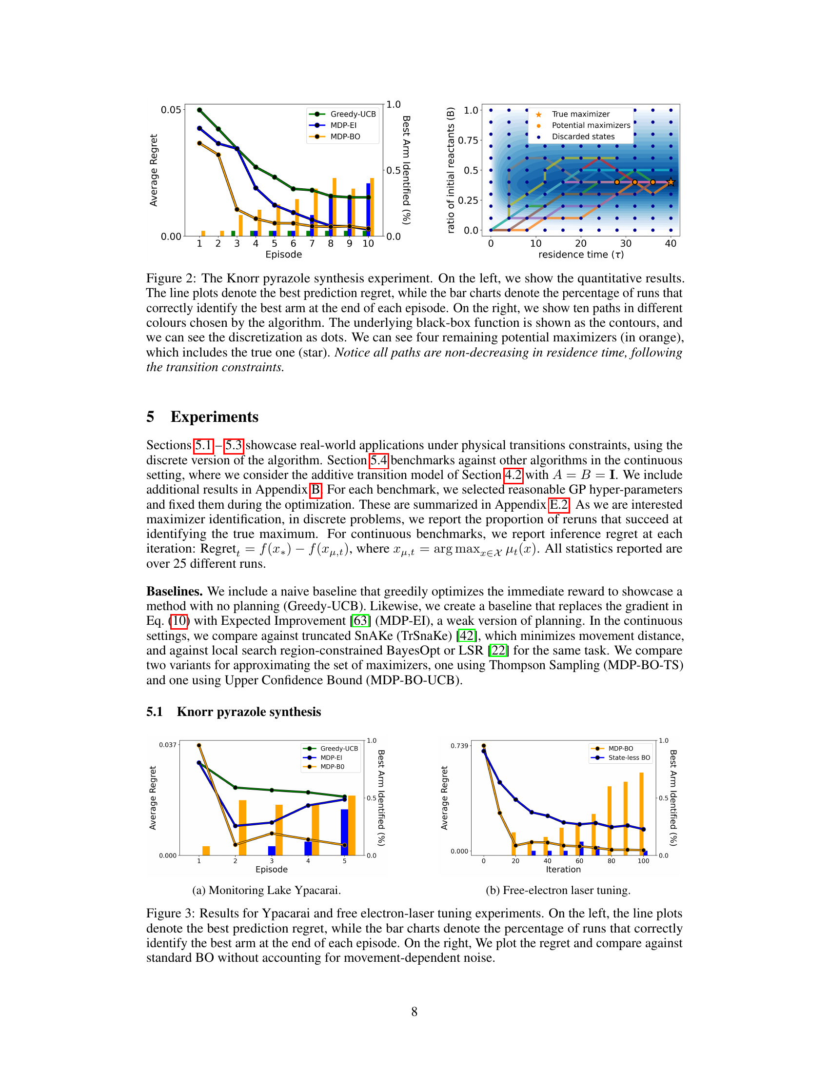
This figure presents the results of two experiments: monitoring Lake Ypacarai and tuning a free-electron laser. The left side shows the average regret (line plot) and the success rate of identifying the best arm (bar chart) over several episodes for both experiments. The right side compares the regret of the proposed method to a standard Bayesian optimization approach that doesn’t consider movement-dependent noise, specifically for the free-electron laser tuning experiment.
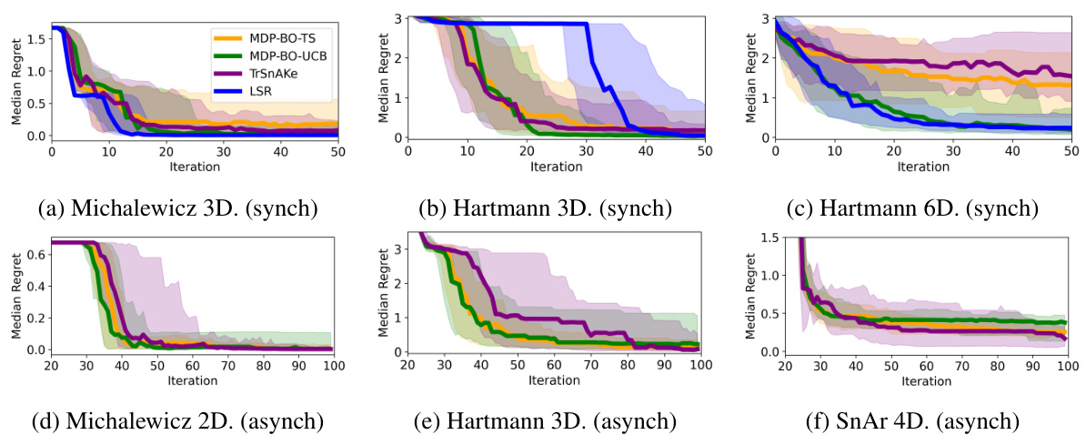
The figure presents the median predictive regret and quantiles for both synchronous and asynchronous benchmarks across six test functions. It compares the performance of MDP-BO-TS, MDP-BO-UCB, TrSnAKe, and LSR, highlighting the effects of different maximization set creation methods and synchronization on the overall performance.
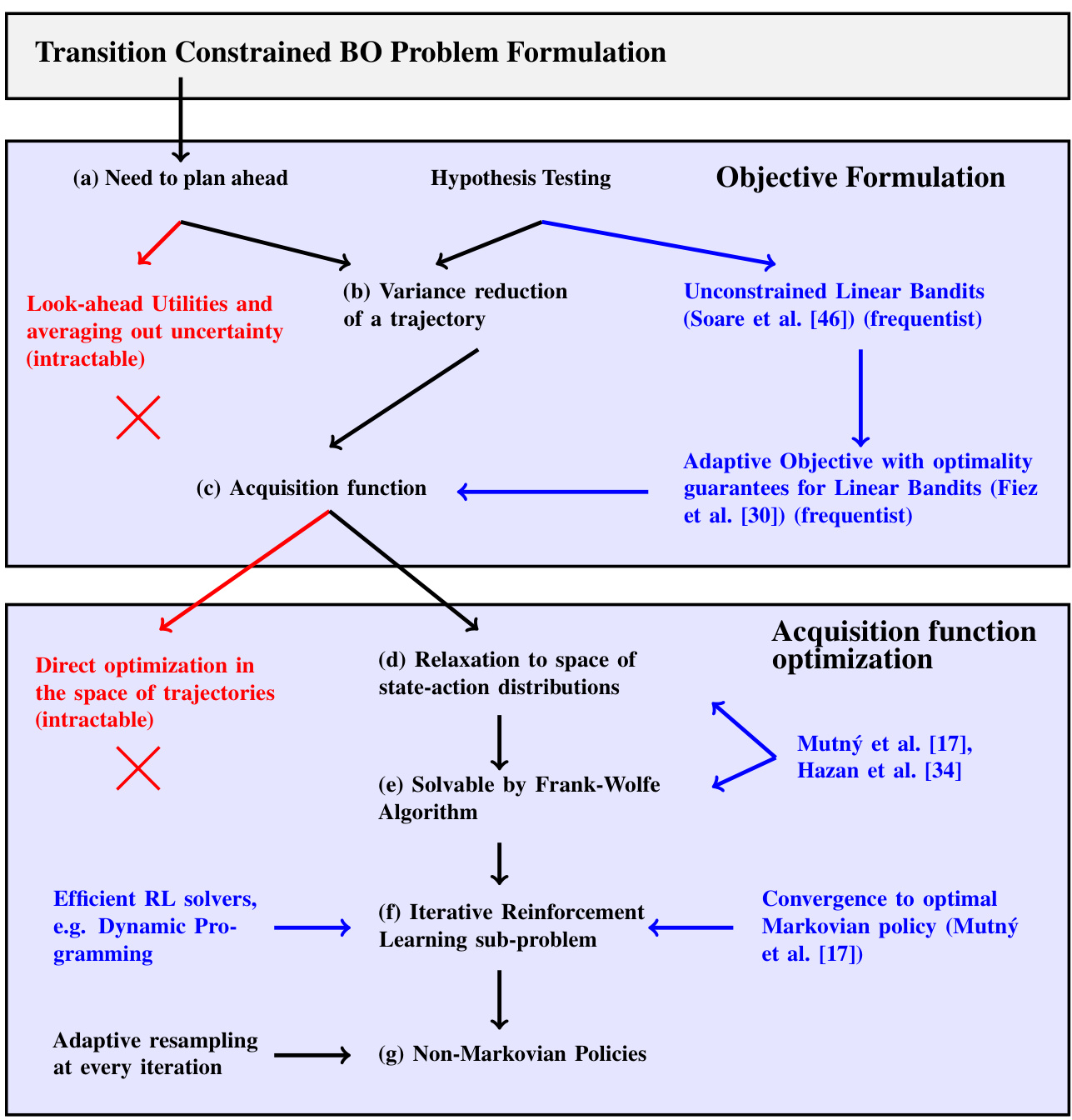
This figure provides a visual summary of the algorithm presented in the paper, highlighting the key steps and their relationships to existing research. It shows how the authors’ approach addresses the challenges of transition-constrained Bayesian optimization by combining elements of hypothesis testing, acquisition function optimization, and reinforcement learning.

This figure presents the results of applying the proposed algorithm to the Knorr pyrazole synthesis experiment. The left side shows the average regret and the success rate of identifying the true maximum over episodes. The right side visualizes ten sample trajectories in the search space, highlighting how the algorithm respects the non-decreasing residence time constraint. The contours represent the true objective function, while the dots show discretized points, indicating the chosen search locations and the remaining potential maximizers.
The figure shows the results of the Knorr pyrazole synthesis experiment using the proposed algorithm. The left panel presents quantitative results showing regret and the percentage of successful maximizer identification. The right panel displays ten different trajectories generated by the algorithm within the constrained search space, with the optimal point and several potential maximizers highlighted.

This figure presents the results of an experiment on the Knorr pyrazole synthesis. The left side shows quantitative results using line plots for best prediction regret and bar charts indicating successful best arm identification. The right side visualizes ten different optimization paths, highlighting the impact of transition constraints by showing that all paths are non-decreasing in residence time. The contours represent the underlying black-box function, and the dots show the discretization.

This figure presents the results of applying the proposed algorithm to the Knorr pyrazole synthesis experiment. The left side shows the average regret (the difference between the true optimal value and the algorithm’s prediction) over multiple runs, comparing it against several baseline methods. The bar charts show the percentage of successful runs in which the algorithm correctly identified the true maximizer. The right side illustrates ten different trajectories (paths) produced by the algorithm in the search space, highlighting their adherence to transition constraints (non-decreasing residence time). The contour plot displays the true underlying black-box function, with dots representing discretized points and the true maximizer marked by a star.

This figure shows the results of a high-noise constrained Ypacarai experiment using immediate feedback. It compares the performance of three different algorithms: Greedy-UCB, MDP-EI, and MDP-BO. The x-axis represents the iteration number, and the y-axis shows the average regret. The shaded areas represent the 10th and 90th percentile ranges. The results indicate that MDP-BO outperforms the other two algorithms in terms of both average regret and the consistency of its performance across multiple runs.

This figure illustrates the Lake Ypacarai environmental monitoring problem with added movement constraints. The lake is represented as a graph, with nodes representing possible measurement locations and edges representing permissible movements between them. Obstacles in the lake restrict movement, creating transition constraints in the optimization problem. The goal is to find the location with the largest contamination (global optimum), indicated by a star, starting from a specified initial state (black square) and ending at a designated final state (dark square). The red line shows the path chosen by the algorithm to navigate the constraints and reach the goal.

This figure presents results from the Knorr pyrazole synthesis experiment. The left side shows quantitative results: best prediction regret over episodes (lines) and the percentage of runs correctly identifying the best arm (bars). The right side visualizes ten different trajectories (colored lines) generated by the algorithm, overlaid on a contour plot of the underlying black-box function and a dot representation of the discretized search space. The paths are constrained to non-decreasing residence times. Four potential maximizers (orange) remain, with the actual maximizer marked with a star.

The figure presents results of the Knorr pyrazole synthesis experiment. The left side shows quantitative results (regret and success rate in identifying the best arm) while the right side visualizes ten different paths followed by the algorithm in the search space. The paths respect the transition constraint of non-decreasing residence time, as shown by the arrows. The contours represent the underlying black-box function, showing the algorithm’s progress towards the true maximizer (star).
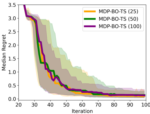
This figure shows an ablation study on the size of the Thompson Sampling maximization set (K) used in the asynchronous Hartmann3D benchmark. The results show that the algorithm’s performance remains consistent across different values of K (25, 50, and 100), suggesting that the choice of K is not a highly sensitive parameter affecting performance.

This figure displays the median predictive regret, along with 10th and 90th percentiles, for asynchronous and synchronous benchmark experiments. It compares the performance of different algorithms (MDP-BO-TS, MDP-BO-UCB, TrSnAKe, and LSR), highlighting the superior performance of Thompson Sampling in asynchronous settings and UCB in synchronous settings. MDP-BO-UCB and LSR show similar strong results.
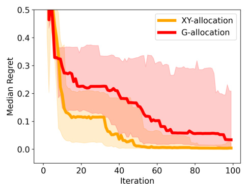
This figure compares the performance of two different allocation methods (XY-allocation and G-allocation) used in the Bayesian Optimization algorithm. Both methods use Thompson Sampling to create maximization sets. While generally showing similar performance, the figure highlights a specific case (Branin2D) where G-allocation significantly underperforms XY-allocation, aligning with findings from the bandit literature.

This figure compares the numerical solution of an ODE (ordinary differential equation) model with an analytical (exact) solution derived from equation 36 in the paper. The purpose is to validate the accuracy of the analytical solution against a numerical approximation. The plot shows the yield over time, with the numerical solution closely tracking the exact solution, demonstrating good agreement between the two approaches.
Full paper#
