TL;DR#
Performative prediction, where a model’s predictions influence the data it’s trained on, is a complex area. Existing optimization methods mostly focus on strongly convex loss functions, limiting their applicability. Non-convex loss functions are more common but harder to analyze. This creates feedback loops that can destabilize training.
This paper tackles this challenge head-on. It introduces a new stationary performative stable (SPS) solution definition for non-convex losses. The authors analyze the convergence of the popular SGD-GD (Stochastic Gradient Descent with Greedy Deployment) method and a novel “lazy” deployment method. They show that while SGD-GD converges to a biased solution, their proposed lazy deployment scheme offers bias-free convergence, leading to more reliable and accurate predictions.
Key Takeaways#
Why does it matter?#
This paper is crucial because it extends the existing performative prediction models to handle non-convex loss functions, a more realistic scenario in many machine learning applications. It provides new theoretical convergence results and opens avenues for future research in this rapidly evolving field, especially regarding the development of novel optimization algorithms and a deeper understanding of the bias-variance trade-off.
Visual Insights#

🔼 This figure shows the results of three different experiments on synthetic data. The left panel displays the SPS measure (||∇J(0t; 0t)||²) against the number of iterations for the SGD-GD algorithm under different sensitivity parameters (ε). The middle panel shows the loss value (J(0t; 0t)) against the number of iterations. The right panel compares the SPS measure of the greedy SGD-GD approach with a lazy deployment strategy, plotting against the number of samples accessed. All experiments use a fixed sensitivity parameter (εL = 2).
read the caption
Figure 1: Synthetic Data (left) SPS measure ||∇J(0t; 0t)||² of SGD-GD against iteration no. t. (middle) Loss value J(0t; 0t) of SGD-GD against iteration no. t. (right) SPS measure ||∇J(0t;0t)||² of greedy (SGD-GD) and lazy deployment against number of sample accessed. We fix EL = 2.

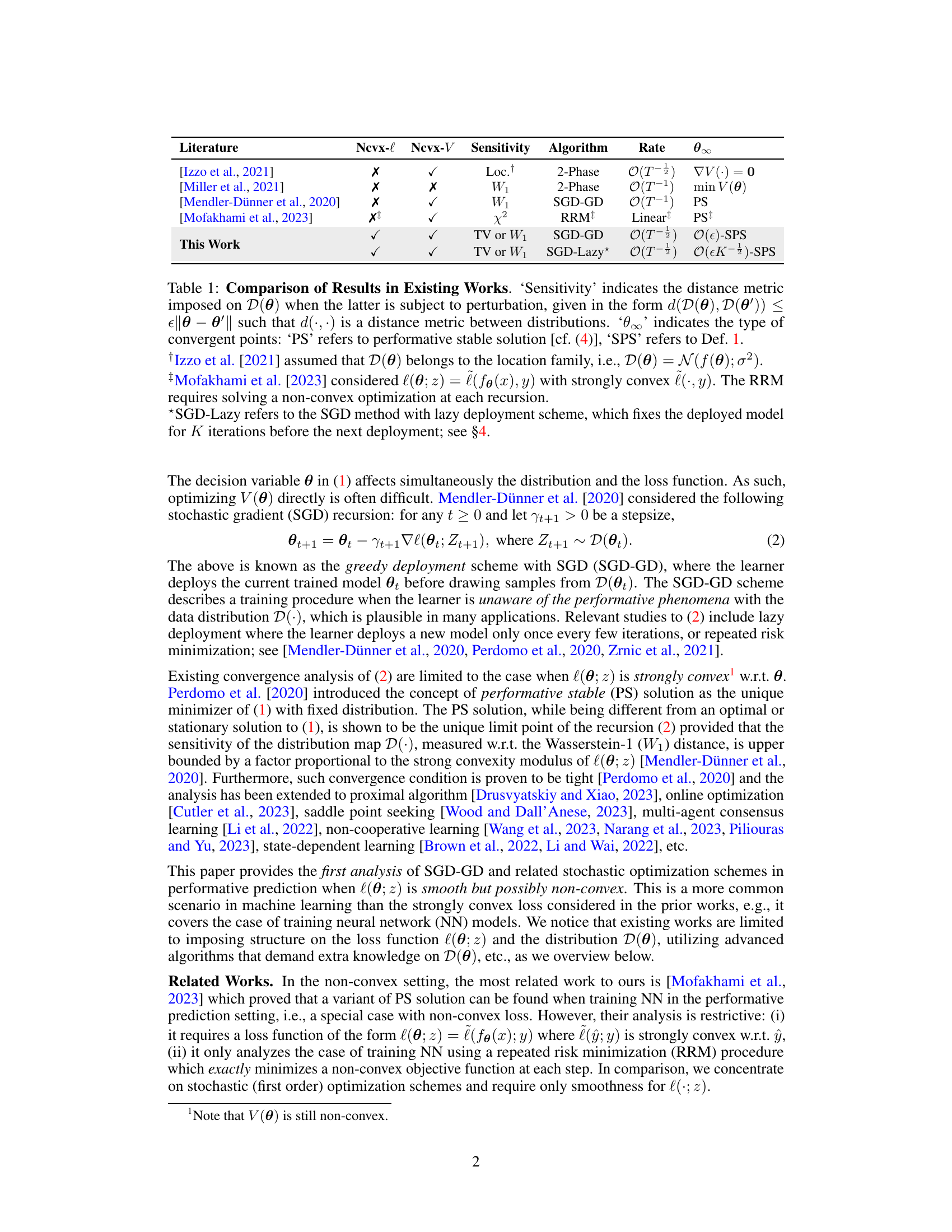
🔼 This table compares the results of this work with existing works on performative prediction. It shows whether the loss function was non-convex in the loss or variance, whether the sensitivity of the data distribution was considered, the algorithm used, its convergence rate, and the type of solution found. The sensitivity metric (e.g., Wasserstein-1 distance, total variation) and the type of solution (performative stable or stationary performative stable) are also listed.
read the caption
Table 1: Comparison of Results in Existing Works. 'Sensitivity' indicates the distance metric imposed on D(θ) when the latter is subject to perturbation, given in the form d(D(θ), D(θ')) ≤ ε||θ – θ'|| such that d(·, ·) is a distance metric between distributions. 'θ∞' indicates the type of convergent points: 'PS' refers to performative stable solution [cf. (4)], 'SPS' refers to Def. 1.
In-depth insights#
Nonconvex Loss SPS#
The concept of ‘Nonconvex Loss SPS’ merges two significant areas in machine learning: nonconvex optimization and performative prediction. Nonconvex loss functions, unlike their convex counterparts, possess multiple local minima, making optimization challenging. Standard gradient descent methods may get stuck in suboptimal solutions. In the context of performative prediction, where a model’s predictions influence the data it’s trained on, this complexity is further amplified. SPS (Stationary Performative Stable) solutions represent a relaxed condition for stability in performative settings; they are points where the gradient of the decoupled performative risk is small, not necessarily zero as in standard optimality conditions. Analyzing convergence to SPS solutions under nonconvex losses is crucial because it provides a more realistic framework for understanding model behavior in practical applications where perfect optimality is often unattainable. The research likely explores novel optimization algorithms or analyses adapted to handle the nonconvexity and convergence to biased SPS solutions, potentially investigating techniques like stochastic gradient descent with lazy updates or other robust optimization methods. The goal is likely to establish conditions under which convergence to an acceptable solution, even if not perfectly optimal, can be guaranteed in this challenging setting.
SGD Convergence#
The convergence analysis of Stochastic Gradient Descent (SGD) in the context of performative prediction is a complex issue due to the inherent feedback loop between model predictions and data distribution. Standard SGD convergence proofs often rely on strong convexity and/or specific assumptions about the data generating process, which are frequently violated in performative settings. The paper likely investigates the convergence properties under relaxed assumptions, potentially addressing non-convex loss functions. Key aspects would involve demonstrating that the algorithm’s iterates approach a stationary point or a performative stable (PS) solution (or a suitably defined variant). The analysis likely involves techniques to manage the bias introduced by the feedback loop, perhaps by bounding the bias and showing that it decreases as the number of iterations increases. A key challenge is that the distribution shift makes typical Lyapunov function arguments difficult. The work likely proposes novel analysis techniques or adapts existing ones (e.g., using time-varying Lyapunov functions) to overcome these challenges. The convergence rate (e.g., sublinear or linear) and the conditions under which convergence is guaranteed are central to the findings. The results may demonstrate convergence to an approximately performative stable (SPS) solution, highlighting the impact of the non-convexity and the feedback loop on the final result. Overall, a thorough understanding of SGD convergence in this setting requires careful consideration of the data-dependent distribution and the unique challenges posed by the performative prediction problem.
Lazy Deployment#
The concept of ’lazy deployment’ in the context of performative prediction offers a pragmatic solution to the challenges of frequent model updates. Traditional approaches deploy a new model after every training iteration, which can be computationally expensive and impractical in real-world scenarios. Lazy deployment addresses this by deferring model updates for a specified number of iterations, reducing the frequency of deployment. This strategy is particularly beneficial when deployment is costly or time-consuming, as seen in applications like spam filtering, where updating the filter frequently may be infeasible. However, this trade-off introduces a bias into the model’s convergence, impacting the accuracy and stability. The analysis within the paper explores how the choice of lazy deployment scheme balances practical constraints with the potential for suboptimal solutions. Theoretical analysis supports the idea that longer lazy deployment epochs leads to convergence to a bias-free solution, while shorter epochs lead to a biased solution. The trade-off between computational efficiency and solution accuracy is a key area of focus, highlighting the need for a balance between deploying too often and too infrequently.
Bias Analysis#
A thorough bias analysis in a machine learning context, especially within the framework of performative prediction, is crucial. It should investigate how the model’s inherent biases interact with the performative feedback loop. This means examining whether the model’s predictions, influenced by its existing biases, systematically alter the data distribution in a way that amplifies or perpetuates those biases. The analysis needs to quantify the magnitude of this bias, ideally separating the bias introduced by the model itself from the bias already present in the initial data. Furthermore, exploring different bias mitigation techniques within the performative prediction setting is key. This could involve studying techniques like data augmentation, algorithmic modifications, or regularization strategies to determine their effectiveness in reducing bias. Finally, the analysis should consider the downstream consequences of biased performative predictions, especially if they have implications for fairness, equity or other societal values.
Future Works#
The “Future Works” section of this research paper could explore several promising avenues. Extending the theoretical analysis to handle more complex scenarios is crucial; this might involve incorporating non-smooth losses, analyzing different data-dependent distribution shift mechanisms beyond the Wasserstein-1 and TV distances, or addressing time-varying sensitivities. Empirical validation on a broader range of real-world datasets across various domains is also necessary to solidify the practical applicability of the proposed methods and explore the limits of their performance. Specifically, it would be beneficial to examine their robustness under different noise levels, data sparsity, and potential model misspecification. Another area of focus could be developing more efficient algorithms. While the paper provides convergence guarantees, the computational complexity of the algorithms could be improved for large-scale applications, perhaps through adaptive step-size techniques or acceleration methods. Finally, investigating practical deployment strategies and their impact on overall system performance is essential. This involves considering factors such as the frequency of model updates, the computational cost of evaluating the performative risk, and the potential for online/offline adaptation. A thorough investigation into these aspects would significantly strengthen the contributions of the work.
More visual insights#
More on figures

🔼 This figure shows the results of three different experiments using synthetic data. The left panel displays the squared norm of the gradient of the decoupled performative risk (||∇J(θt;θt)||²) over iterations for SGD-GD with different sensitivity parameters (ε). The middle panel shows the loss function (J(θt;θt)) for the same experiments. The right panel compares the performance of the greedy (SGD-GD) and lazy deployment schemes in terms of ||∇J(θt;θt)||² against the number of data samples accessed.
read the caption
Figure 1: Synthetic Data (left) SPS measure ||∇J(θt;θt)||² of SGD-GD against iteration no. t. (middle) Loss value J(θt;θt) of SGD-GD against iteration no. t. (right) SPS measure ||∇J(θt;θt)||² of greedy (SGD-GD) and lazy deployment against number of sample accessed. We fix εL = 2.
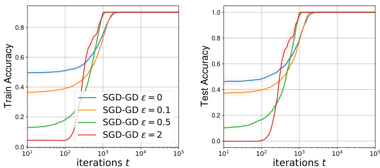
🔼 This figure shows the results of experiments using synthetic data. The left panel displays the SPS measure (||∇J(θt; θt)||²) over iterations for SGD-GD under different sensitivity parameters (ε). The middle panel shows the loss function values (J(θt; θt)) over iterations for the same experiment. The right panel compares the SPS measure for both greedy (SGD-GD) and lazy deployment strategies showing how the number of samples accessed affects the SPS measure. The experiments use εL = 2.
read the caption
Figure 1: Synthetic Data (left) SPS measure ||∇J(θt; θt)||² of SGD-GD against iteration no. t. (middle) Loss value J(θt; θt) of SGD-GD against iteration no. t. (right) SPS measure ||∇J(θt; θt)||² of greedy (SGD-GD) and lazy deployment against number of sample accessed. We fix εL = 2.

🔼 This figure shows three plots comparing the performance of SGD-GD and lazy deployment in a synthetic data experiment. The left plot shows the SPS measure (||∇J(θt;θt)||²) against the iteration number (t). The middle plot shows the loss (J(θt;θt)) against the iteration number (t). The right plot shows the SPS measure against the number of samples accessed. The εL parameter was fixed at 2 for all experiments.
read the caption
Figure 1: Synthetic Data (left) SPS measure ||∇J(θt;θt)||² of SGD-GD against iteration no. t. (middle) Loss value J(θt;θt) of SGD-GD against iteration no. t. (right) SPS measure ||∇J(θt;θt)||² of greedy (SGD-GD) and lazy deployment against number of sample accessed. We fix εL = 2.

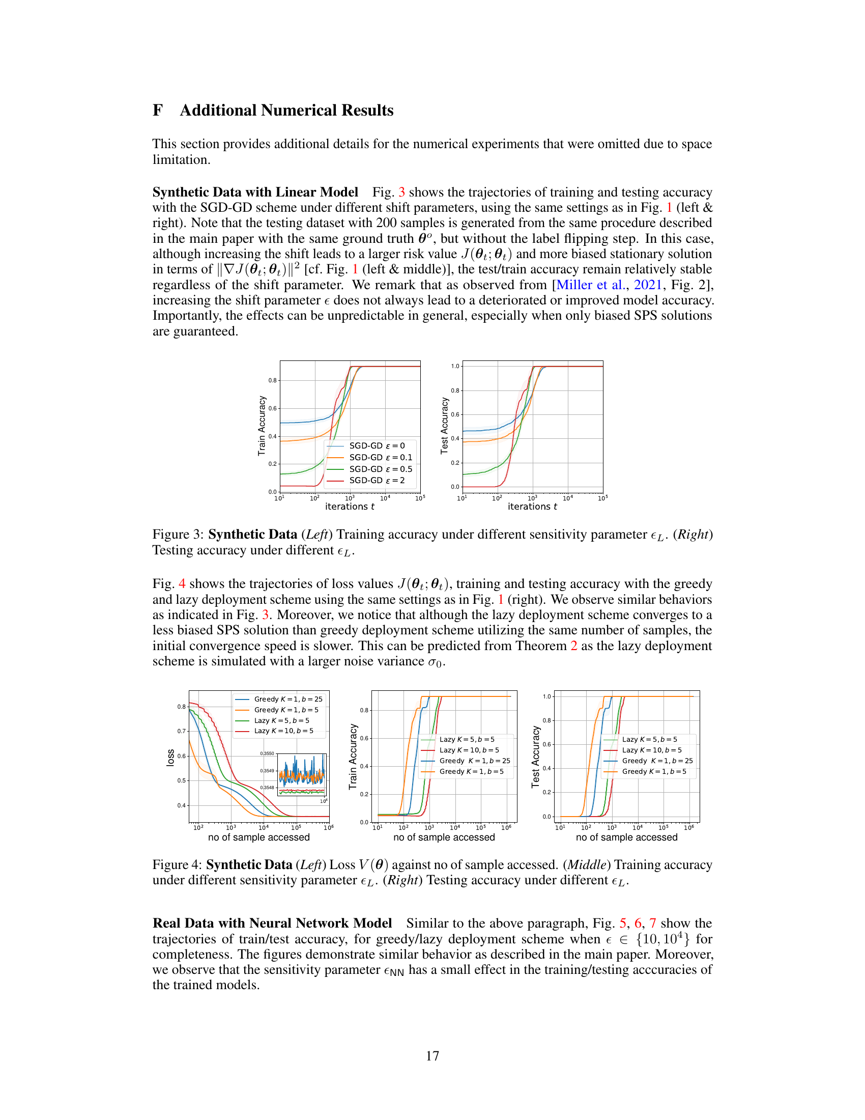
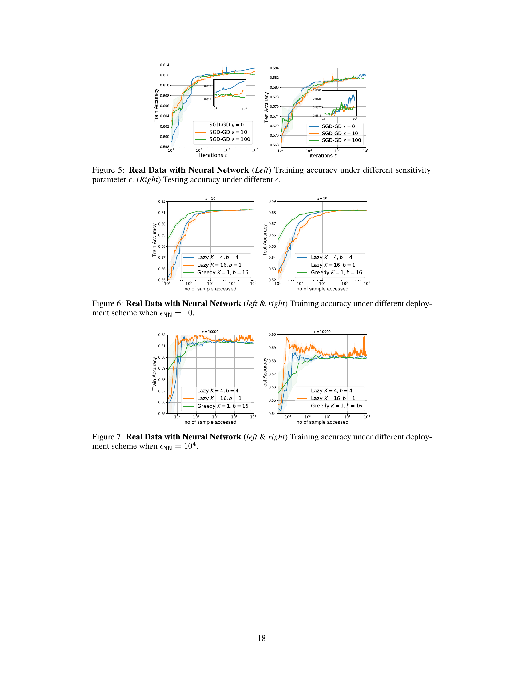
🔼 This figure shows the training and testing accuracy of a neural network model trained using the SGD-GD algorithm with different sensitivity parameters (ε). The left panel displays the training accuracy, while the right panel shows the testing accuracy. The results indicate that increasing the sensitivity parameter leads to a slight decrease in both training and testing accuracy, demonstrating that higher sensitivity in the data distribution can have a negative impact on the model’s performance.
read the caption
Figure 5: Real Data with Neural Network (Left) Training accuracy under different sensitivity parameter ε. (Right) Testing accuracy under different ε.
🔼 This figure presents the results of experiments on synthetic data using a linear model with a sigmoid loss function. Three subfigures show different aspects of the SGD-GD optimization algorithm and a lazy deployment variant. The left panel shows the convergence of the squared norm of the decoupled performative gradient to a stationary point over iterations, illustrating the algorithm’s convergence behavior toward a stationary performative stable solution. The middle panel shows the convergence of the loss function itself. The right panel compares the greedy and lazy deployment schemes, highlighting the impact of the number of samples accessed on the convergence towards a bias-free SPS solution. The experiments help in verifying the theoretical findings presented in the paper regarding the convergence rates and bias levels of different deployment schemes.
read the caption
Figure 1: Synthetic Data (left) SPS measure ||∇J(0t; 0t)||² of SGD-GD against iteration no. t. (middle) Loss value J(0t; 0t) of SGD-GD against iteration no. t. (right) SPS measure ||∇J(0t;0t)||2 of greedy (SGD-GD) and lazy deployment against number of sample accessed. We fix EL = 2.
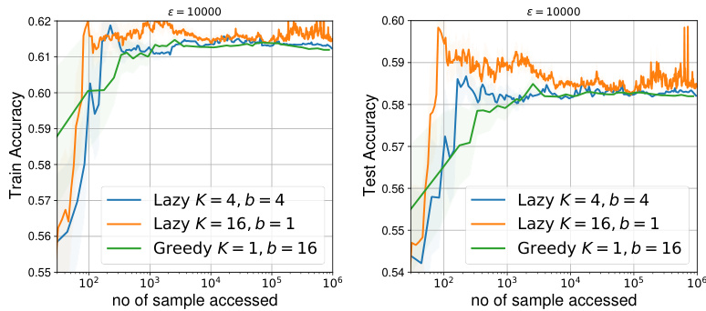
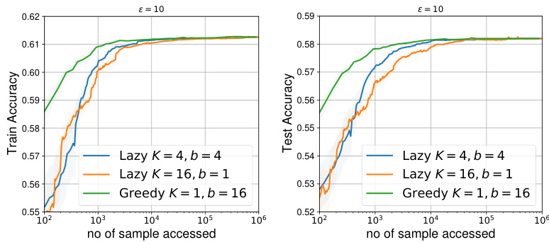
🔼 This figure displays the results of experiments using real-world data and a neural network model to perform performative prediction. The left panel shows how the SPS measure (a measure of convergence to a stationary point) changes over iterations (t) for the SGD-GD algorithm under varying sensitivity parameters (εnn). The middle and right panels illustrate how the SPS measure evolves as a function of the number of samples accessed for both greedy (SGD-GD) and lazy deployment strategies, with sensitivity parameters εnn set to 10 and 10000, respectively. This visualization helps compare the convergence behavior and bias levels of these different approaches.
read the caption
Figure 2: Real Data with Neural Network Benchmarking with SPS measure ||∇J(θt; θt)||². (left) Against t for SGD-GD with parameters εnn ∈ {0, 10, 100}. (middle & right) Against no. of samples with greedy (SGD-GD) and lazy deployment when εnn = 10 & εnn = 10⁴, respectively.
Full paper#
