↗ OpenReview ↗ NeurIPS Homepage ↗ Chat
TL;DR#
Mobile health interventions often struggle with personalization due to user variability and changing contexts. Existing bandit algorithms often fail to effectively adapt to these dynamic conditions. This results in suboptimal interventions, leading to missed opportunities for positive health outcomes.
The researchers address this by introducing RoME, a novel robust mixed-effects contextual bandit algorithm. RoME incorporates user and time-specific random effects, network cohesion penalties, and flexible baseline reward estimation. This comprehensive approach allows RoME to handle participant heterogeneity and non-stationarity effectively. The algorithm’s superior performance is validated through rigorous simulations and real-world mHealth studies, demonstrating its practical applicability and potential to significantly improve the effectiveness of personalized health interventions.
Key Takeaways#
Why does it matter?#
This paper is crucial for researchers in mobile health and reinforcement learning due to its novel algorithm, RoME. RoME tackles challenges like user heterogeneity and non-stationary rewards that hinder existing algorithms. Its superior performance, backed by theoretical analysis and real-world studies, makes it a valuable tool for personalizing mHealth interventions and optimizing other contextual bandit applications.
Visual Insights#

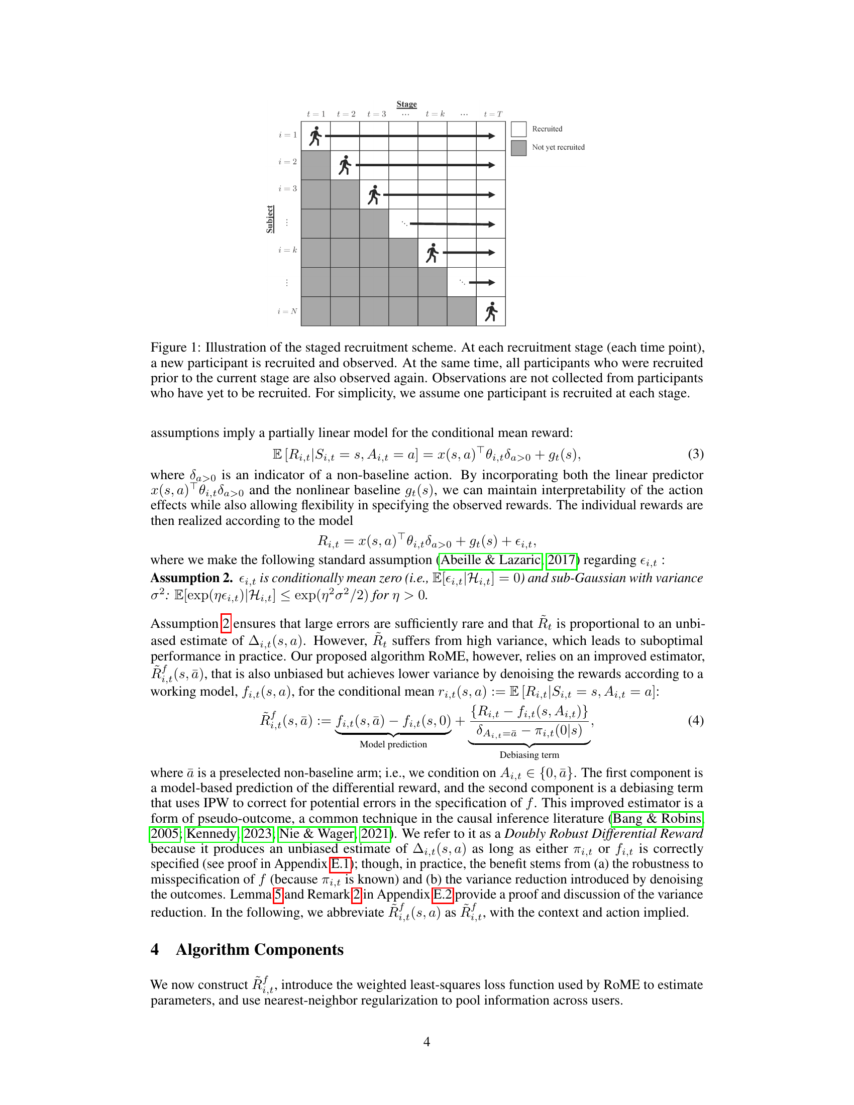
This figure illustrates the staged recruitment process used in the study. New participants are added at each stage, and data is collected on all previously recruited participants at each stage. This creates a triangular data structure where the number of observations increases with each stage.

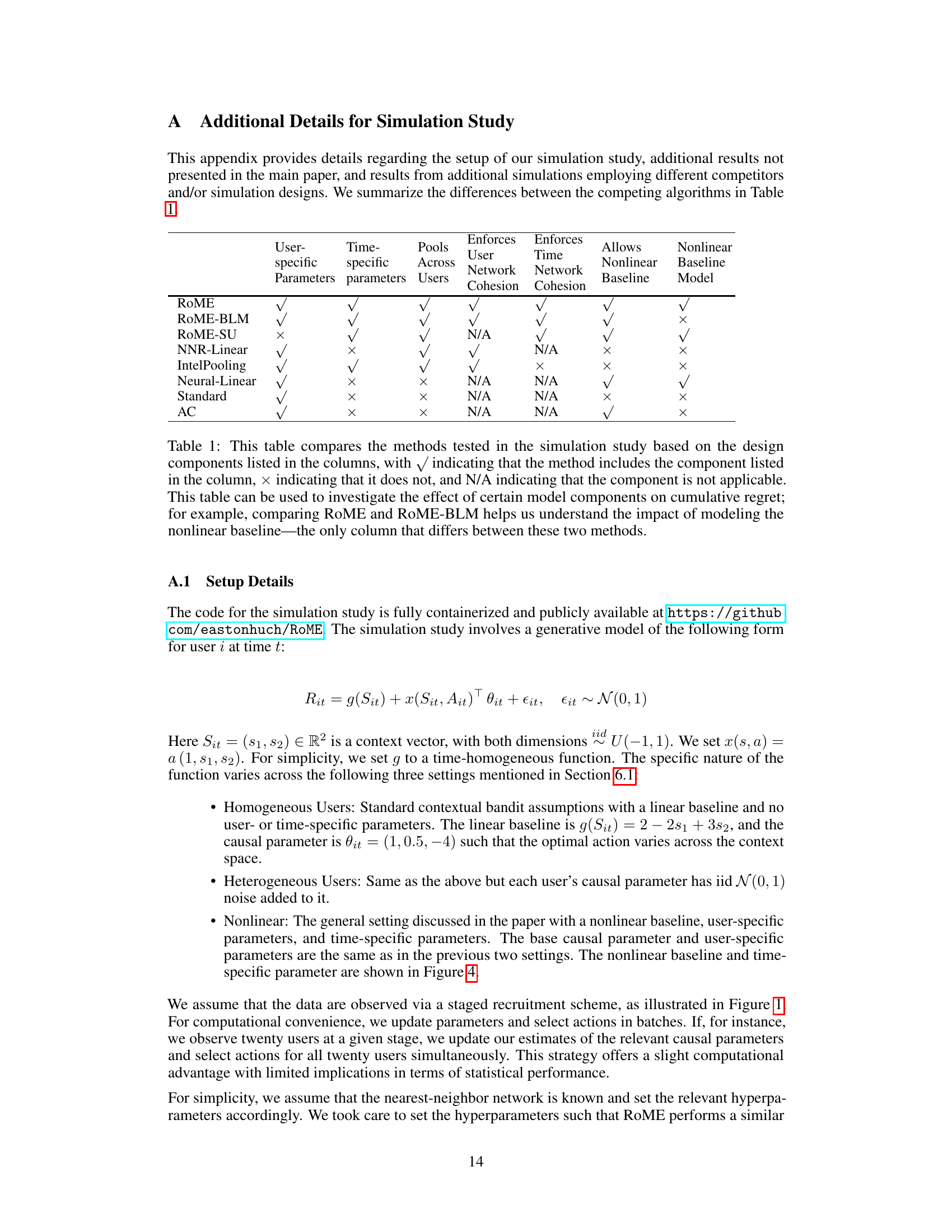
This table compares the eight methods used in the simulation study, highlighting the presence or absence of key features: user-specific parameters, time-specific parameters, pooling across users, user network cohesion, time network cohesion, a nonlinear baseline, and a nonlinear baseline model. It helps understand how these features affect the cumulative regret, a measure of the algorithm’s performance.
In-depth insights#
RoME’s Robustness#
RoME’s robustness stems from its multifaceted design. Modeling differential rewards with user- and time-specific random effects directly addresses participant heterogeneity and non-stationarity, common challenges in mHealth interventions. Network cohesion penalties improve performance by efficiently pooling information across users and time, further mitigating the effects of noisy data. The utilization of debiased machine learning enhances the flexibility and reliability of reward estimation, even in scenarios with complex baseline reward structures. These three key components, combined with a proven Thompson sampling algorithm, make RoME resilient to various forms of data noise and model misspecification, yielding robust regret bounds and overall superior performance compared to other methods.
Mixed-Effects Model#
The concept of a mixed-effects model is crucial for analyzing data where observations are clustered or nested within groups, capturing both within-group and between-group variations. In the context of the provided research paper, a mixed-effects model is likely employed to account for heterogeneity among users. This model incorporates both fixed effects, representing average treatment effects, and random effects, representing individual variations in treatment response. The random effects help model individual user differences in baseline reward, reflecting participant heterogeneity and improving the model’s accuracy and robustness. The time-varying nature of the data might also be incorporated by including time-specific random effects within the mixed-effects model, further enhancing its capacity to model the dynamic nature of treatment effects over time. Ultimately, the utilization of a mixed-effects contextual bandit algorithm allows for more accurate and personalized treatment strategies by effectively capturing the complex interplay of individual differences, contexts, and time-dependent effects.
Debiased Learning#
Debiased machine learning, in the context of this research paper, is crucial for accurately estimating the treatment effects in mobile health interventions. The core idea is to create an estimator that is robust to misspecifications in the model used to predict the conditional mean reward. This is achieved by incorporating a debiasing term into the estimation process. This debiasing term helps correct for errors arising from model misspecification, leading to more reliable estimates of treatment effects even when the model for baseline rewards is highly complex. The paper highlights the importance of using techniques like doubly robust methods which offer a degree of protection against bias caused by inaccurate model assumptions. Combining these debiasing methods with flexible machine learning techniques, like random forests, ensures the estimation is sufficiently accurate and can handle diverse reward distributions and nonstationary behavior. The primary advantage of this approach lies in maintaining unbiasedness and achieving robustness, leading to reliable and accurate results that are less dependent on assumptions about the complexity of the baseline reward function. This enhanced accuracy translates into improved decision-making about personalized interventions for better health outcomes.
Regret Bound Analysis#
Regret bound analysis in reinforcement learning, and specifically in the context of contextual bandits, is crucial for evaluating algorithm performance. A tight regret bound provides a theoretical guarantee on the algorithm’s performance, quantifying how far its cumulative reward falls short of the optimal strategy. The paper likely focuses on deriving a high-probability regret bound, establishing a strong theoretical foundation for the proposed RoME algorithm. This involves carefully analyzing the algorithm’s behavior under various conditions, including user heterogeneity, non-stationarity, and complex reward models. The bound’s dependence on key factors like model dimension, instead of the complexity of the baseline reward, is likely highlighted, showcasing RoME’s robustness. The analysis probably leverages techniques from concentration inequalities and martingale theory to control stochastic fluctuations and establish a high-probability bound, signifying that the algorithm achieves the stated regret with a high degree of certainty. The obtained bound helps demonstrate the algorithm’s efficiency and its practical applicability, ultimately validating RoME’s effectiveness in mobile health settings.
Future Directions#
The research paper’s ‘Future Directions’ section would ideally explore several promising avenues. Extending RoME to handle non-linear treatment effects more robustly is crucial, potentially leveraging advanced machine learning techniques beyond the current DML framework. Investigating data-adaptive methods for hyperparameter tuning and network construction would enhance RoME’s adaptability across diverse mHealth applications. Addressing the long-term effects of interventions, such as treatment fatigue or evolving user behavior, through dynamic modeling approaches would improve real-world relevance. Developing efficient computational strategies is vital for enabling large-scale deployments and facilitating real-time optimization in dynamic settings. Finally, rigorous exploration of privacy-preserving techniques for integrating sensitive personal data is essential for ethical and responsible application of such powerful algorithms in mHealth.
More visual insights#
More on figures

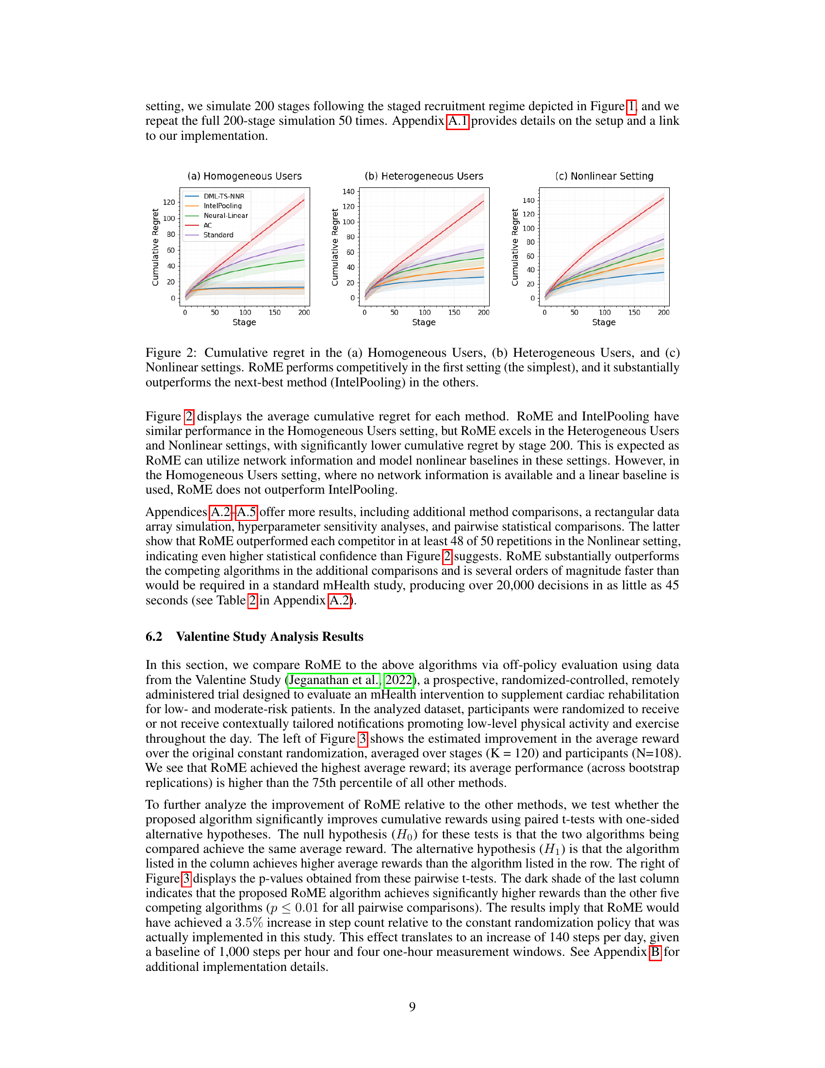
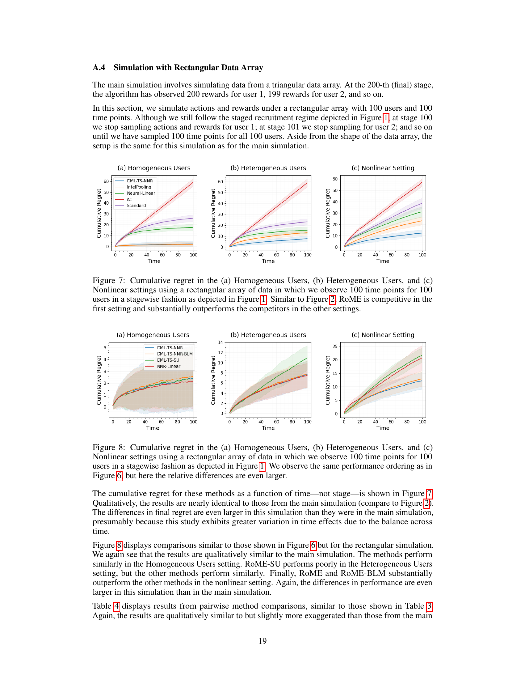
This figure displays the average cumulative regret for four different contextual bandit algorithms across three simulation settings: homogeneous users, heterogeneous users, and nonlinear setting. The x-axis represents the stage of the simulation, and the y-axis represents the cumulative regret. The plot shows that RoME is competitive with other methods in the simplest setting (homogeneous users), but significantly outperforms them in the more complex settings (heterogeneous and nonlinear).

The left panel of the figure displays boxplots of the unbiased estimates of the average per-trial rewards for five different contextual bandit algorithms, including RoME, relative to the rewards obtained using a pre-specified randomization policy. The right panel shows a heatmap of p-values from pairwise paired t-tests comparing the performance of these five algorithms.

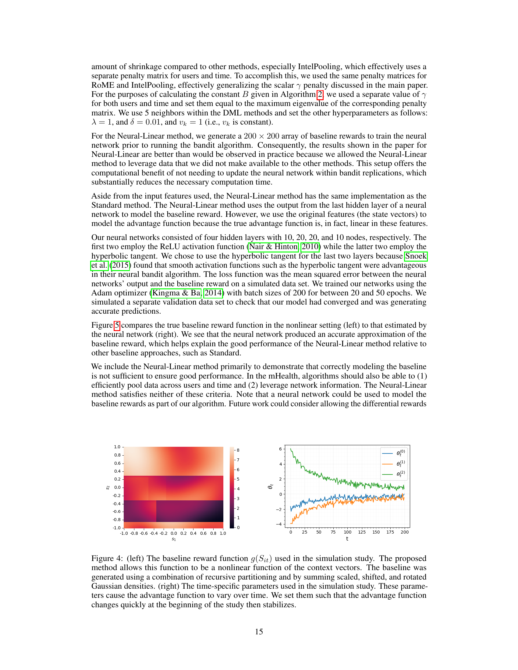
The left panel shows a heatmap representing the nonlinear baseline reward function used in the simulation. This function’s complexity highlights the challenge addressed by the RoME algorithm. The right panel displays the time-varying parameters incorporated in the simulation, illustrating how these parameters influence the treatment effect (differential reward) over time. These parameters are designed to change significantly at the beginning of the study before stabilizing later.

This figure compares the cumulative regret of RoME against four other bandit algorithms across three different simulation settings: homogeneous users, heterogeneous users, and nonlinear settings. The x-axis represents the stage of the simulation, and the y-axis represents the cumulative regret. The results show that RoME performs competitively in the simplest setting (homogeneous users), but significantly outperforms the other algorithms in the more complex settings (heterogeneous users and nonlinear settings). This demonstrates RoME’s robustness and superior performance in scenarios with user heterogeneity and non-linear relationships between context and reward.

This figure displays the average cumulative regret for four different bandit algorithms across three different simulation settings: homogeneous users, heterogeneous users, and nonlinear settings. The x-axis represents the stage of the simulation, and the y-axis represents the cumulative regret. The figure shows that the RoME algorithm performs competitively with other algorithms in the simple homogeneous setting but significantly outperforms other algorithms in the more complex heterogeneous and nonlinear settings.

This figure displays the average cumulative regret for four different contextual bandit algorithms across three different simulation settings: Homogeneous Users, Heterogeneous Users, and Nonlinear. The algorithms compared are RoME, IntelPooling, Neural-Linear, Action-Centered (AC), and Standard Thompson Sampling. The results show that RoME performs competitively in the simplest setting (Homogeneous Users), but significantly outperforms the other algorithms in the more complex settings (Heterogeneous Users and Nonlinear). The shaded areas represent the standard deviation across 50 simulations.

This figure displays the cumulative regret for four different bandit algorithms across three distinct simulation settings: Homogeneous Users, Heterogeneous Users, and Nonlinear. The x-axis represents the stage of the simulation (time), and the y-axis represents the cumulative regret. Each line represents a different algorithm (RoME, IntelPooling, Neural-Linear, AC, and Standard). The shaded regions around the lines represent confidence intervals. The figure demonstrates that the RoME algorithm performs comparably to the other algorithms in the simplest setting (Homogeneous Users) but significantly outperforms them in the more complex settings (Heterogeneous Users and Nonlinear), particularly in terms of cumulative regret.

This figure shows the time heterogeneity in the treatment effects from the Valentine study. The pseudo-outcomes were calculated, averaged across participants, and plotted over time. The resulting curve shows substantial variation in the treatment effects over the course of the study, indicating a non-stationary effect.

This figure displays a boxplot showing the unbiased estimates of the average per-trial reward for three algorithms: RoME, RoME-SU (RoME without user-specific effects), and NNR-Linear (network-cohesion bandit algorithm). The estimates are relative to the reward obtained under the pre-specified Valentine Study randomization policy. The boxplot is accompanied by a heatmap displaying the p-values from pairwise paired t-tests, comparing the performance of the three algorithms.

The left panel shows the boxplots of unbiased reward estimates for five algorithms in the Valentine study, comparing their performance relative to a standard randomization policy. The right panel provides a heatmap showing p-values from paired t-tests comparing the average reward of each pair of algorithms. The results indicate whether the differences are statistically significant.
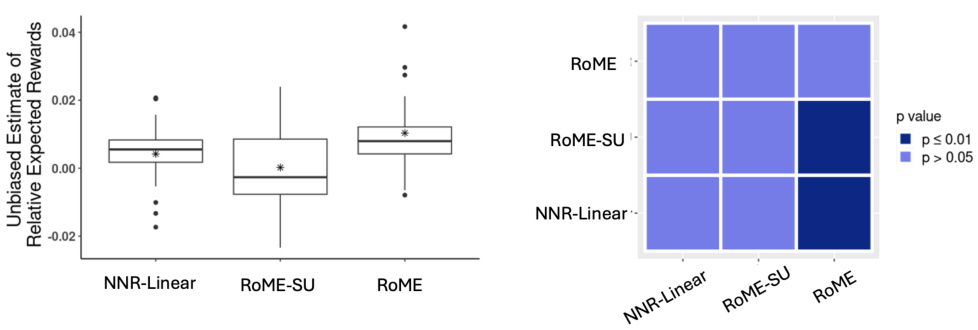
This figure displays the results of an ablation study comparing three variations of the RoME algorithm: RoME, RoME-SU (without user-specific effects), and NNR-Linear (without DML). The left panel shows boxplots of the unbiased estimates of the average per-trial reward for each algorithm, relative to a control (Valentine Study randomization policy). The asterisk (*) indicates the mean. The right panel shows p-values from pairwise paired t-tests comparing the algorithms. Darker shading indicates statistical significance at the p ≤ 0.01 level.
More on tables
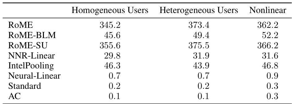
This table shows the average computation time of different contextual bandit algorithms across three different simulation settings (Homogeneous Users, Heterogeneous Users, and Nonlinear). The settings vary in complexity and the algorithms’ ability to handle these complexities. The table highlights the computational efficiency of RoME and RoME-BLM compared to other algorithms. While RoME and RoME-SU require slightly longer computation time, they are still significantly faster than the time required for actual mHealth study deployments. NNR-Linear and IntelPooling have lower computation time but may compromise performance compared to RoME in more complex scenarios.

This table compares eight different methods used in a simulation study, highlighting their key features and components related to user-specific and time-specific parameters, network cohesion, and nonlinear baseline modeling. It also helps in understanding how different components affect the cumulative regret.

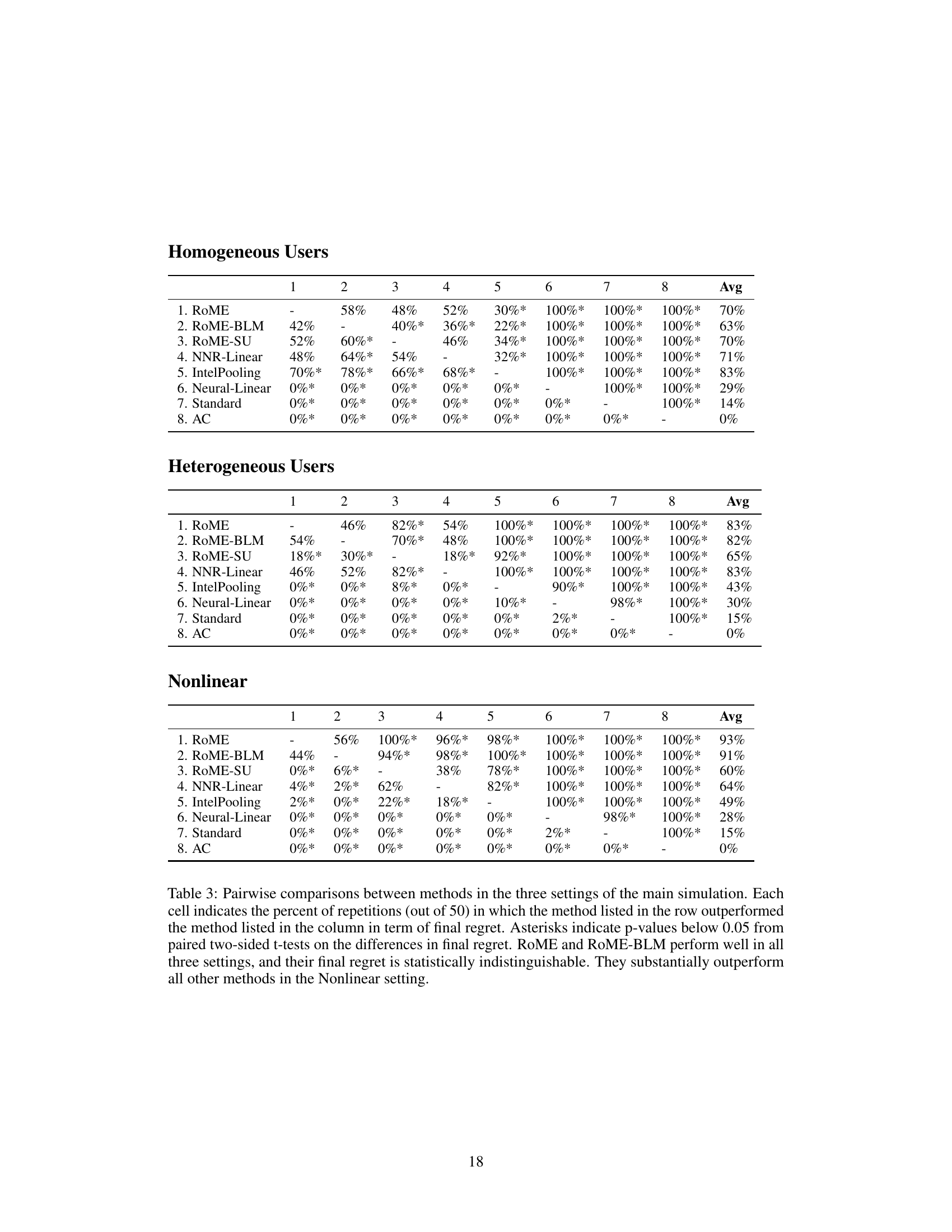
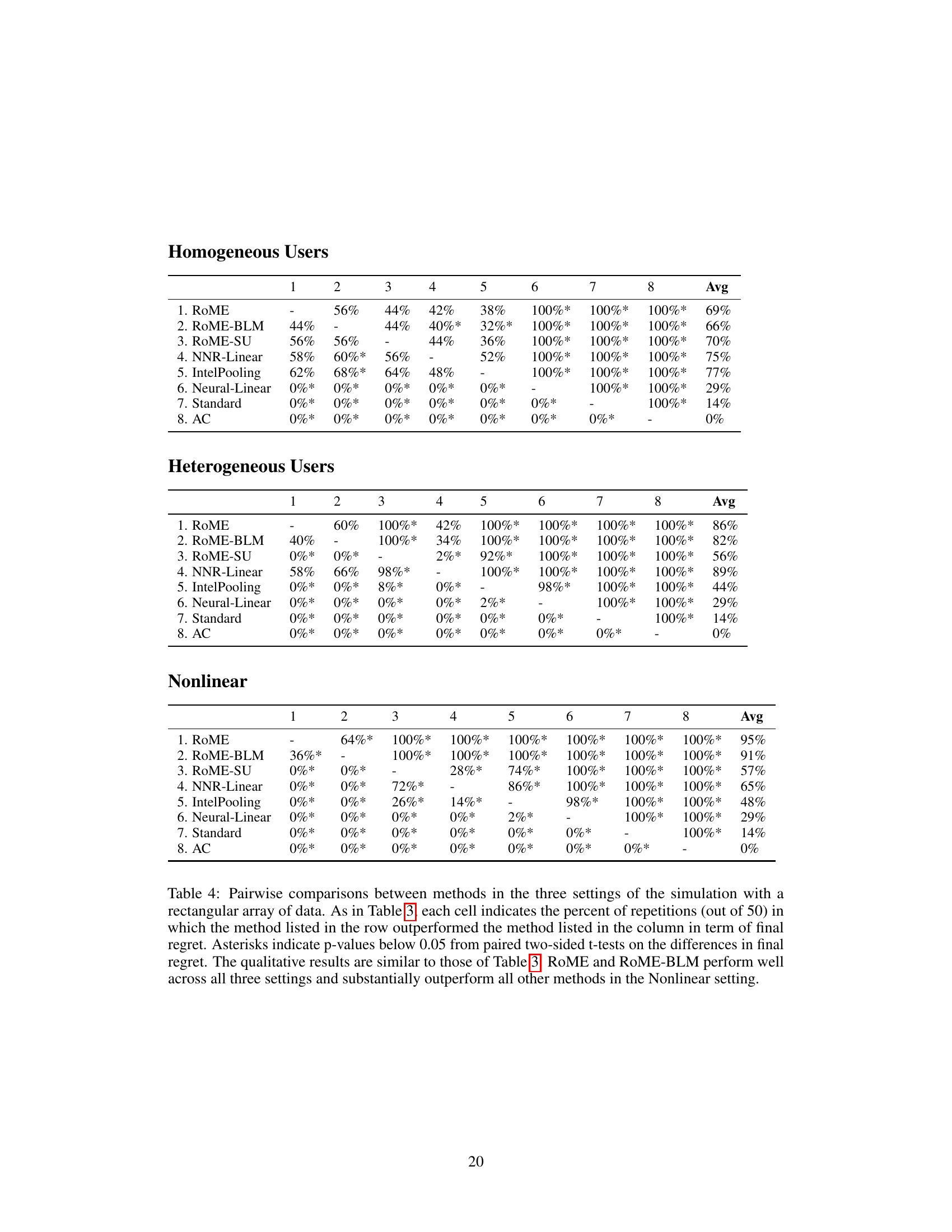
This table presents the results of pairwise comparisons between different methods across three settings (Homogeneous Users, Heterogeneous Users, Nonlinear) in a simulation study. The percentage of times each method outperformed another method in terms of cumulative regret is shown. Statistical significance (p<0.05) is indicated with asterisks. RoME and RoME-BLM consistently perform well and are statistically indistinguishable, significantly outperforming others in the complex Nonlinear setting.

This table presents the results of pairwise comparisons between eight different methods across three different settings (Homogeneous Users, Heterogeneous Users, and Nonlinear Setting) in a simulation study. The comparison is based on the percentage of times each method outperformed another in terms of final regret. Statistical significance (p<0.05) is indicated. RoME and RoME-BLM generally perform very well, particularly in the most complex setting.

This table compares eight different methods used in a simulation study. Each method is evaluated based on several design choices, indicated by checkmarks and crosses in the table. The comparison helps to understand how different model components affect the cumulative regret, which is a measure of the algorithm’s performance.

This table presents pairwise comparisons between eight different methods across three different settings (Homogeneous Users, Heterogeneous Users, and Nonlinear) using the percentage of times each method outperformed the others. It shows RoME and RoME-BLM consistently perform well across all settings, with statistically significant outperformance against others in the nonlinear setting. The table highlights the robust nature of RoME across diverse conditions.

This table presents the results of pairwise comparisons between different methods across three simulation settings (Homogeneous Users, Heterogeneous Users, and Nonlinear). Each cell shows the percentage of times one method outperformed another, based on 50 repetitions. Asterisks indicate statistically significant differences (p<0.05). The results highlight the consistent strong performance of RoME and RoME-BLM, particularly in the more complex Nonlinear setting.

This table compares eight methods used in the simulation study, highlighting which design components each method includes. It aids in understanding the influence of various model components on cumulative regret by comparing similar methods that differ by only one component.

This table displays the results of pairwise comparisons between eight different methods across three different settings (Homogeneous Users, Heterogeneous Users, and Nonlinear Setting) in a simulation study. Each cell shows the percentage of times one method outperformed another based on final regret. Asterisks indicate statistical significance (p<0.05). The results highlight that RoME and RoME-BLM generally perform very well, especially in the complex nonlinear setting, significantly outperforming other methods.

This table presents the results of pairwise comparisons between eight different methods (RoME, ROME-BLM, ROME-SU, NNR-Linear, IntelPooling, Neural-Linear, Standard, AC) across three settings (Homogeneous Users, Heterogeneous Users, Nonlinear). For each pair of methods within each setting, it shows the percentage of simulation runs where one method outperformed the other. Asterisks indicate statistically significant differences (p<0.05) based on paired t-tests. RoME and ROME-BLM consistently perform well, especially in the challenging Nonlinear setting.

This table compares eight different methods used in a simulation study. Each method is evaluated based on whether it incorporates several key design components: user-specific parameters, time-specific parameters, pooling across users, network cohesion penalties, and the inclusion of nonlinear baseline models. The table helps to understand how these different components affect the cumulative regret (a measure of algorithm performance).

This table presents the results of an ANOVA test performed on the pseudo-outcomes from the Valentine study. The analysis investigates whether treatment effects vary significantly across participants and over time. The extremely low p-values (less than 2e-16 for participants and 4e-04 for weeks) strongly indicate that both participant-level and time-dependent factors significantly influence treatment effects. This supports the use of mixed-effects models that incorporate these individual and temporal variations.

This table compares eight different methods used in a simulation study, highlighting their key characteristics and features. Each method is evaluated based on whether it incorporates user-specific and time-specific parameters, network cohesion, and the use of a nonlinear baseline model. The table helps in understanding how these components influence the overall performance of the methods and allows for a focused comparison between them.
Full paper#
