TL;DR#
Mixed time series (MiTS) data, comprising continuous and discrete variables, are prevalent in various real-world applications yet under-explored in current time series analysis. Existing methods struggle because the different variable types exhibit different temporal patterns and distributions, leading to insufficient and imbalanced representation learning. Ignoring this heterogeneity results in biased and inaccurate analysis.
The proposed MiTSformer framework addresses these limitations by introducing two key inductive biases: 1) it recovers latent continuous variables (LCVs) underlying the discrete variables (DVs) by hierarchically aggregating multi-scale temporal information and leveraging adversarial guidance from continuous variables (CVs); 2) it fully captures spatial-temporal dependencies through cascaded self- and cross-attention blocks. This approach demonstrates consistent state-of-the-art performance across five MiTS analysis tasks, showing the effectiveness of addressing data heterogeneity for improved analytical results.
Key Takeaways#
Why does it matter?#
This paper is important because it tackles the largely unexplored problem of analyzing mixed time series (MiTS), which contain both continuous and discrete data. MiTS are common in various fields but existing methods often struggle due to data heterogeneity. This work introduces a novel framework that effectively addresses this issue, opening new avenues for research and applications.
Visual Insights#

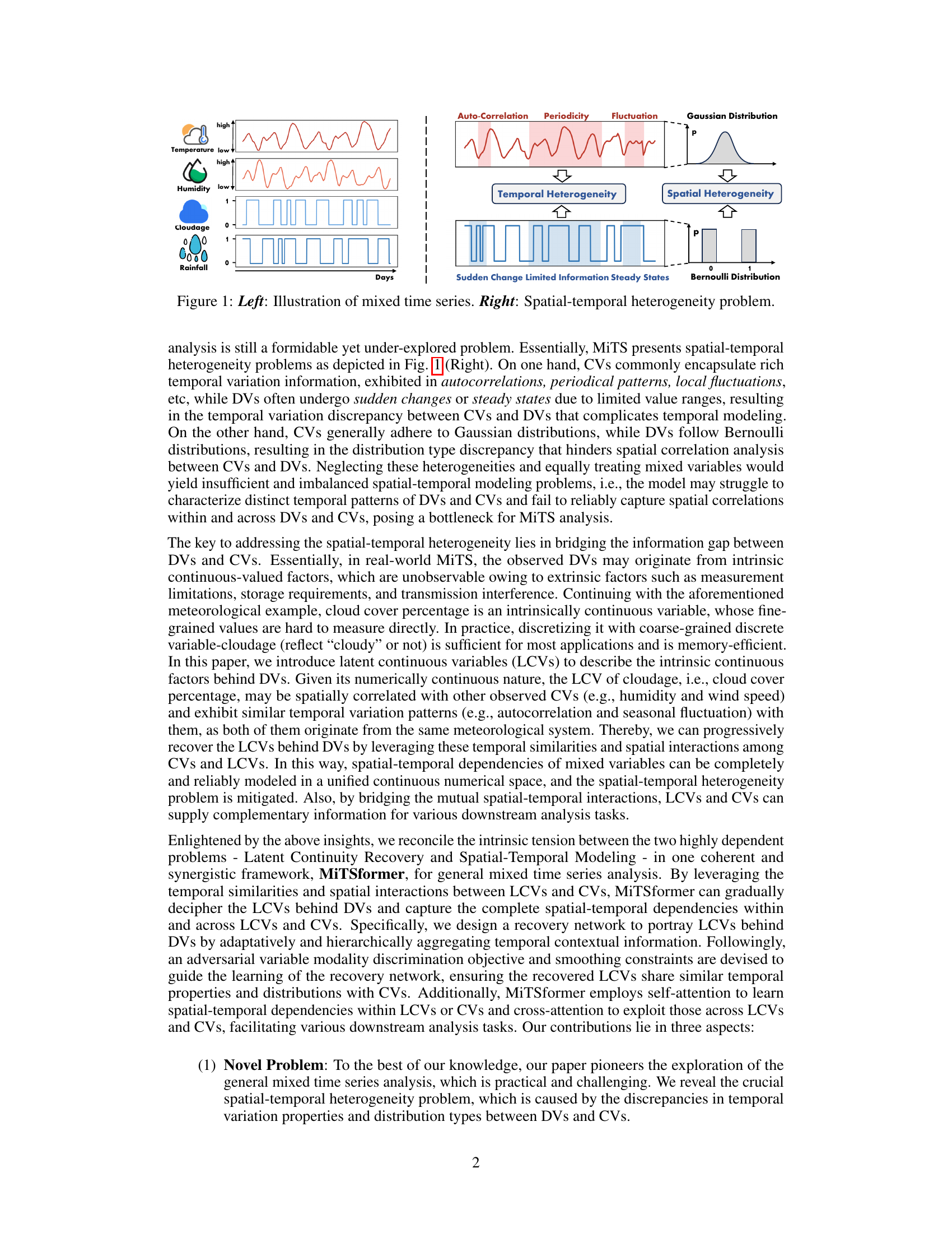
🔼 The figure illustrates the concept of mixed time series and highlights the challenges posed by spatial-temporal heterogeneity. The left panel shows an example of a mixed time series, with continuous variables (temperature and humidity) exhibiting smooth, continuous patterns, and discrete variables (cloudage and rainfall) showing abrupt changes and distinct distributions. The right panel visually depicts the problem of spatial-temporal heterogeneity, emphasizing the differences in temporal patterns and distributions between the continuous and discrete variables, which complicate the process of building effective models for analysis.
read the caption
Figure 1: Left: Illustration of mixed time series. Right: Spatial-temporal heterogeneity problem.

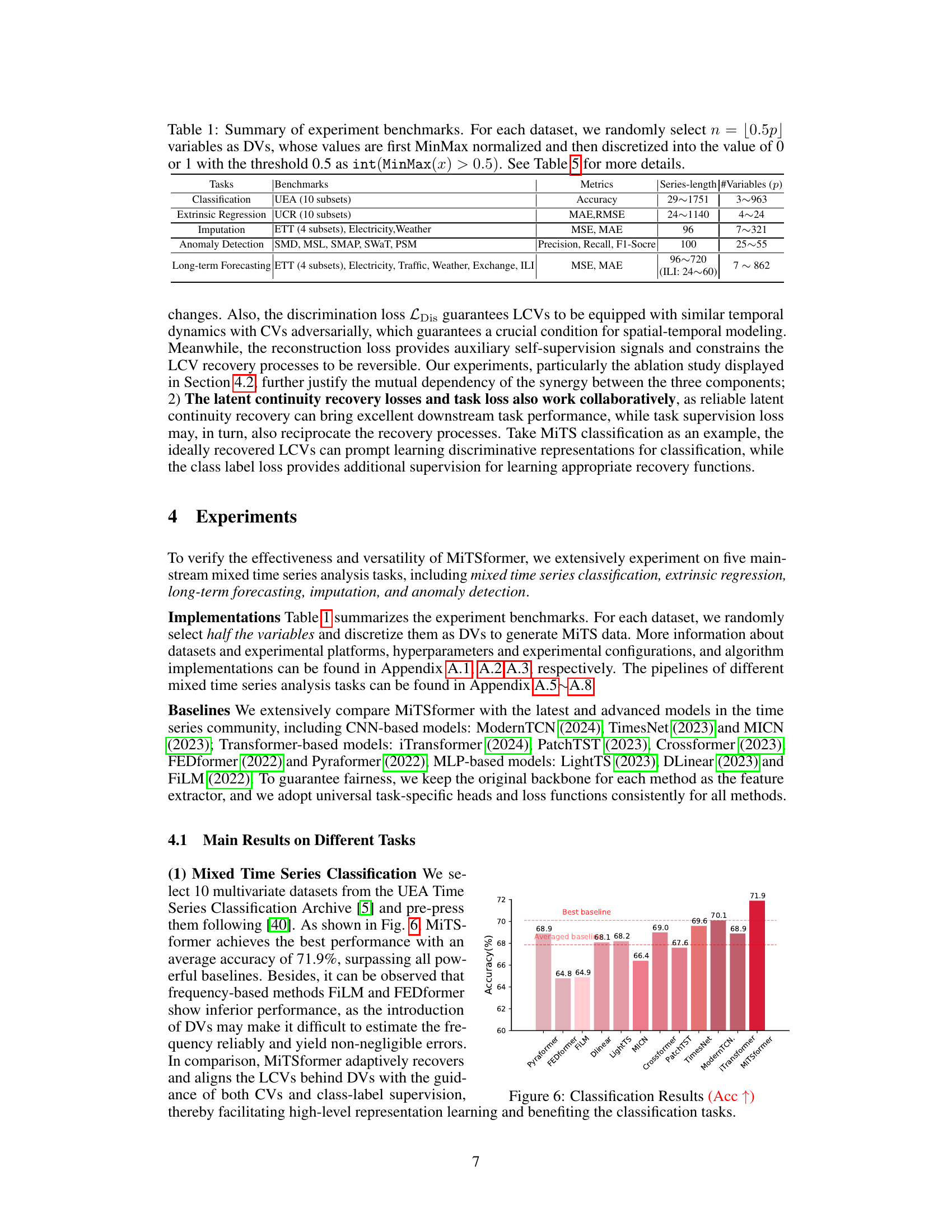
🔼 This table summarizes the benchmark datasets used in the experiments for five different mixed time series analysis tasks: classification, extrinsic regression, imputation, anomaly detection, and long-term forecasting. For each task, it lists the benchmark dataset used, the metrics used for evaluation, and the range of series lengths and number of variables (p) in the datasets. The table also notes that for each dataset, half of the variables (n = 0.5p) were randomly selected and converted to discrete variables (DVs) through a MinMax normalization and discretization process.
read the caption
Table 1: Summary of experiment benchmarks. For each dataset, we randomly select n = [0.5p] variables as DVs, whose values are first MinMax normalized and then discretized into the value of 0 or 1 with the threshold 0.5 as int(MinMax(x) > 0.5). See Table 5 for more details.
In-depth insights#
MiTS Heterogeneity#
MiTS (Mixed Time Series) heterogeneity presents a significant challenge in time series analysis due to the inherent differences between continuous and discrete variables. Continuous variables (CVs) often exhibit rich temporal dynamics, while discrete variables (DVs) may have limited temporal information, potentially originating from underlying continuous variables through discretization. This disparity in temporal patterns can lead to imbalanced representation learning. Furthermore, CVs and DVs often follow different probability distributions, further hindering the effectiveness of standard time series models. Successfully addressing MiTS heterogeneity requires innovative techniques that can bridge the information gap between CVs and DVs, perhaps by recovering the latent continuous information within DVs and modelling the spatial and temporal interactions between the two variable types. A key insight is to recognize that the discrete nature of DVs might be an artifact of measurement constraints rather than an inherent characteristic of the underlying process. Therefore, recovering the latent continuous representation of DVs and using them along with CVs to build a robust model capable of capturing complete spatial-temporal dependencies is a crucial step.
LCV Recovery Net#
A hypothetical “LCV Recovery Net” in a time series analysis paper would likely focus on recovering latent continuous variables (LCVs) from observed discrete variables (DVs). The core challenge is that DVs often lose fine-grained information due to the discretization process. The network would aim to reconstruct these LCVs, potentially utilizing techniques like convolutional neural networks (CNNs) or recurrent neural networks (RNNs) to capture temporal dependencies. Adversarial training, using continuous variables (CVs) as a guide, might be incorporated to ensure the recovered LCVs align with the overall temporal patterns of the data. This would create a more complete and balanced representation, improving the accuracy of downstream tasks like classification or forecasting. The effectiveness of the LCV Recovery Net would depend heavily on the quality of the adversarial training and the ability of the chosen architecture to effectively model complex temporal dynamics and relationships between LCVs and CVs.
Attention Blocks#
Attention blocks are crucial in the MiTSformer architecture for capturing complex spatial-temporal dependencies within and across mixed time series data. They are cascaded, meaning the output of one block feeds into the next, allowing for progressively refined representations. The architecture uses two key types of attention blocks: self-attention, which focuses on relationships within a single variable modality (CVs or recovered LCVs), and cross-attention, which captures interactions between the two modalities. This dual-attention approach enables the model to effectively learn both intra- and inter-variable relationships, a significant advantage over methods that treat CVs and DVs uniformly. The adaptive learning of aggregation processes through adversarial guidance further enhances the effectiveness of the attention mechanism by ensuring sufficient and balanced representation learning for all variable types. The use of both self- and cross-attention is key to the success of MiTSformer, enabling comprehensive modeling of spatial-temporal heterogeneity in mixed time series data.
Empirical Results#
The empirical results section of a research paper is crucial for validating the claims made in the introduction and methodology. A strong empirical results section will present a comprehensive evaluation of the proposed method’s performance on various tasks and datasets, typically comparing it to relevant baselines. Key aspects of a thoughtful empirical results section include a clear description of the experimental setup, datasets used, and metrics employed. The results should be presented in a way that is easy to understand and interpret, using tables, figures, and other visualizations as appropriate. Statistical significance should be properly addressed to show the reliability of the findings. Furthermore, an in-depth analysis should be conducted to explain the observed results, highlighting both successes and limitations. A robust empirical results section substantially increases the credibility and impact of a research paper, ultimately determining its acceptance or rejection.
Future Research#
Future research directions stemming from this work on mixed time series analysis could involve several key areas. Extending the model’s capabilities to handle diverse data types, beyond continuous and binary, is crucial. This would require investigating techniques for incorporating categorical or ordinal variables effectively. Further, exploring advanced pre-training methods to leverage large language models (LLMs) and enhance the model’s generalizability and efficiency could unlock significant improvements, particularly in cases with limited data. The development of more sophisticated techniques for handling missing data and noisy signals will be vital. This includes investigating novel imputation methods specifically designed for mixed time series. Finally, application to larger-scale, real-world datasets and the development of robust evaluation metrics for various downstream tasks will be key to translating the research into practical applications. Addressing these challenges will allow for more accurate and versatile mixed time series analysis in a wide range of domains.
More visual insights#
More on figures

🔼 This figure illustrates the relationships between observed discrete variables (DVs), observed continuous variables (CVs), and latent continuous variables (LCVs). It highlights that DVs originate from underlying continuous variables (LCVs) but lose fine-grained information due to external interference factors (like measurement limitations or discretization). The figure emphasizes the two key insights used in the MiTSformer model: 1. Temporal Similarity: LCVs and CVs share similar temporal patterns (autocorrelation, periodicity, trends). 2. Spatial Interaction: LCVs and CVs interact spatially and influence each other’s values. By leveraging these similarities and interactions, the MiTSformer aims to recover the LCVs from the DVs, enabling more accurate and complete spatial-temporal modeling.
read the caption
Figure 2: Connections among DVs, CVs, and LCVs.

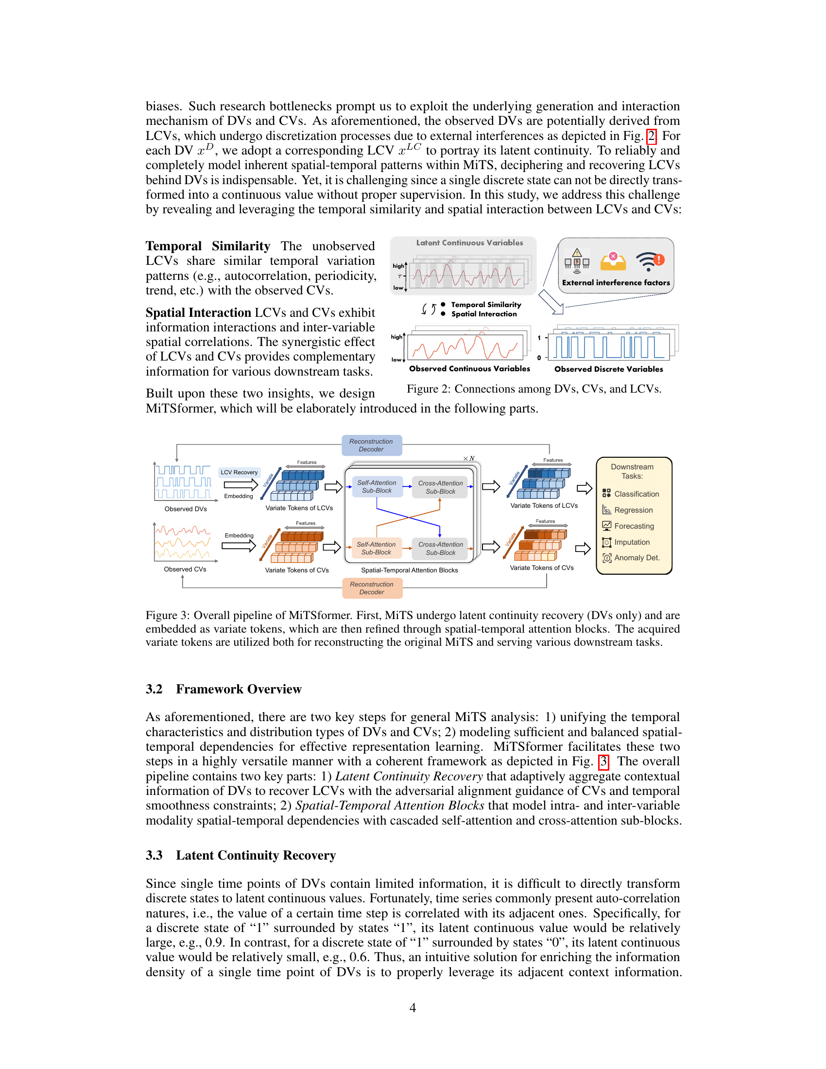
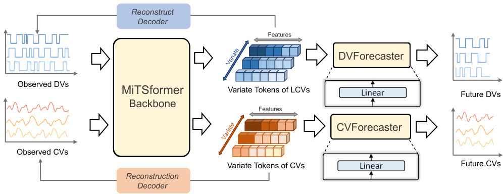
🔼 The figure shows the overall architecture of the MiTSformer model. It begins with latent continuity recovery for the discrete variables (DVs), which are then embedded and processed alongside the continuous variables (CVs). Both DVs and CVs are fed into spatial-temporal attention blocks to capture dependencies. The outputs are used for reconstructing the original mixed time series and for various downstream tasks (classification, regression, forecasting, imputation, and anomaly detection).
read the caption
Figure 3: Overall pipeline of MiTSformer. First, MiTS undergo latent continuity recovery (DVs only) and are embedded as variate tokens, which are then refined through spatial-temporal attention blocks. The acquired variate tokens are utilized both for reconstructing the original MiTS and serving various downstream tasks.
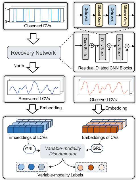
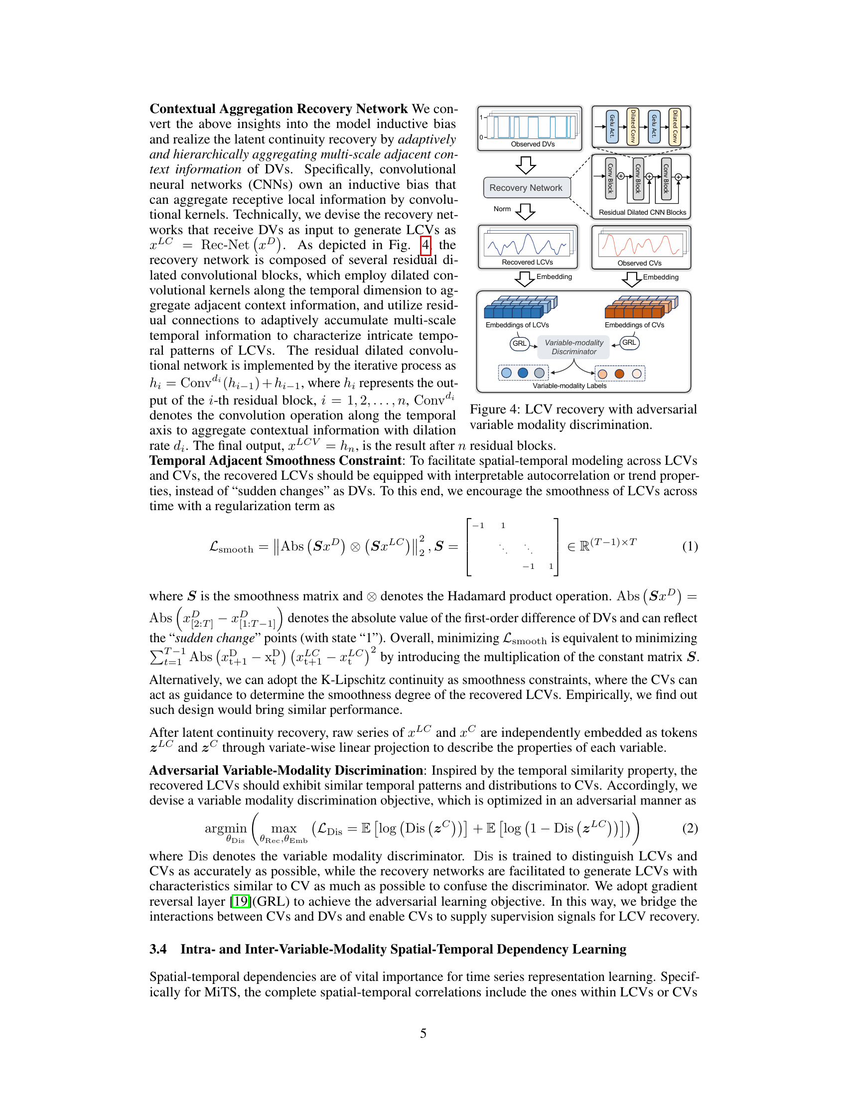
🔼 This figure shows the architecture of the Latent Continuity Recovery network in MiTSformer. It uses a recovery network composed of residual dilated convolutional blocks to recover LCVs from DVs. It also incorporates an adversarial variable modality discrimination component that uses a discriminator to distinguish between embeddings of LCVs and CVs. The goal is to ensure that recovered LCVs have temporal patterns and distributions similar to CVs.
read the caption
Figure 4: LCV recovery with adversarial variable modality discrimination.

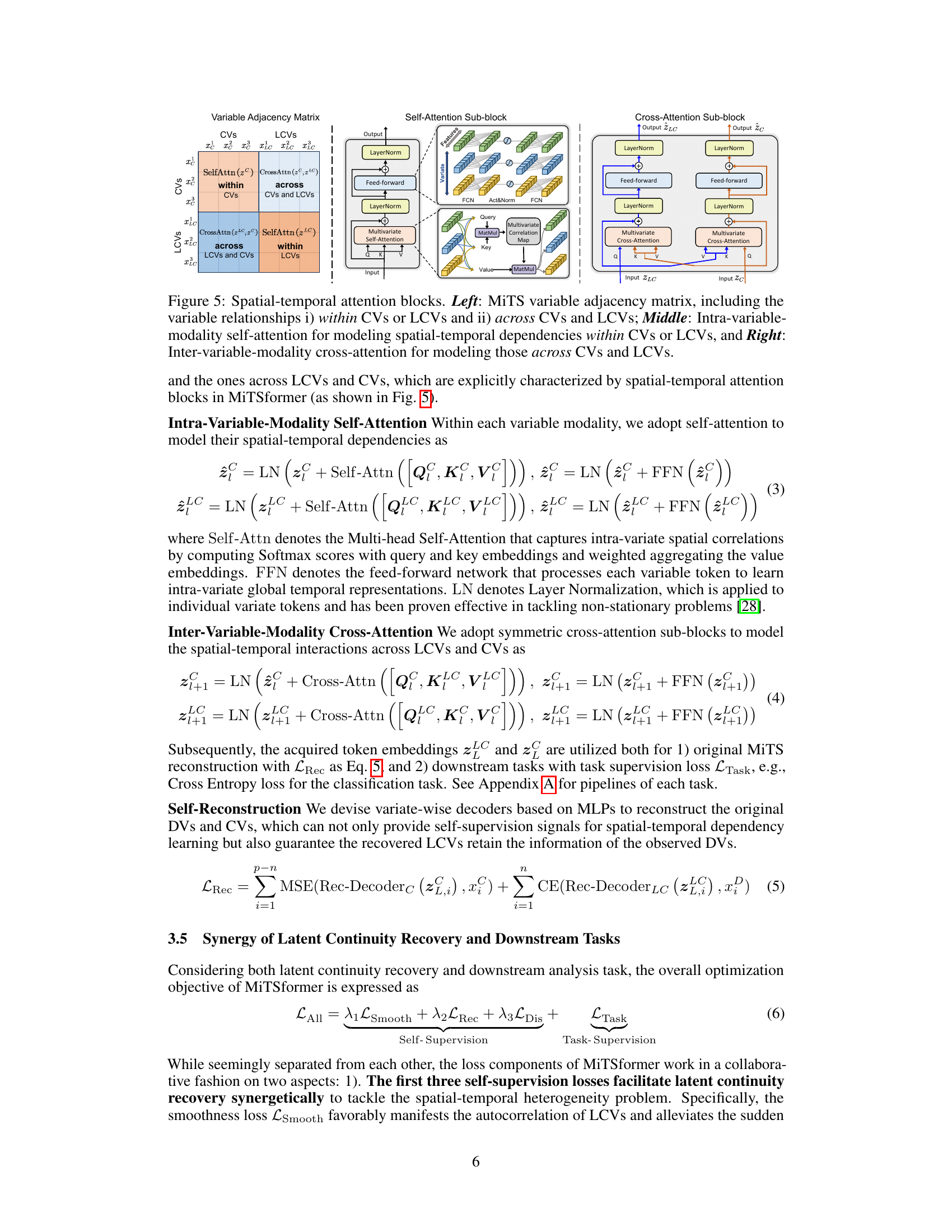
🔼 This figure illustrates the architecture of the spatial-temporal attention blocks in MiTSformer. The left panel shows the variable adjacency matrix, representing the relationships between continuous variables (CVs), latent continuous variables (LCVs), and discrete variables (DVs) within and across modalities. The middle panel details the intra-modality self-attention mechanism used to model spatial-temporal relationships within each modality (CVs or LCVs). The right panel depicts the inter-modality cross-attention mechanism used to model relationships between CVs and LCVs.
read the caption
Figure 5: Spatial-temporal attention blocks. Left: MiTS variable adjacency matrix, including the variable relationships i) within CVs or LCVs and ii) across CVs and LCVs; Middle: Intra-variable-modality self-attention for modeling spatial-temporal dependencies within CVs or LCVs, and Right: Inter-variable-modality cross-attention for modeling those across CVs and LCVs.

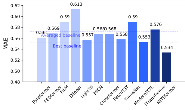
🔼 This figure shows the classification accuracy results for different models on 10 datasets from the UEA archive. MiTSformer achieves the best overall performance, significantly outperforming other methods, including frequency-based models that struggle with the introduction of discrete variables. The results highlight MiTSformer’s ability to effectively model spatial-temporal patterns in mixed time series.
read the caption
Figure 6: Classification Results (Acc↑)
🔼 This figure illustrates the architecture of the spatial-temporal attention blocks used in the MiTSformer model. The left panel shows the variable adjacency matrix, which represents the relationships between variables within each modality (CVs or LCVs) and across modalities. The middle panel details the intra-variable modality self-attention mechanism, used to capture spatial-temporal dependencies within a single modality. The right panel depicts the inter-variable modality cross-attention mechanism, designed to capture dependencies between the CVs and LCVs.
read the caption
Figure 5: Spatial-temporal attention blocks. Left: MiTS variable adjacency matrix, including the variable relationships i) within CVs or LCVs and ii) across CVs and LCVs; Middle: Intra-variable-modality self-attention for modeling spatial-temporal dependencies within CVs or LCVs, and Right: Inter-variable-modality cross-attention for modeling those across CVs and LCVs.
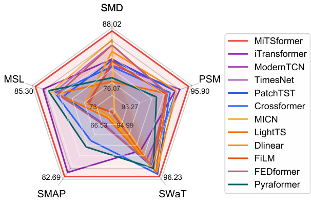
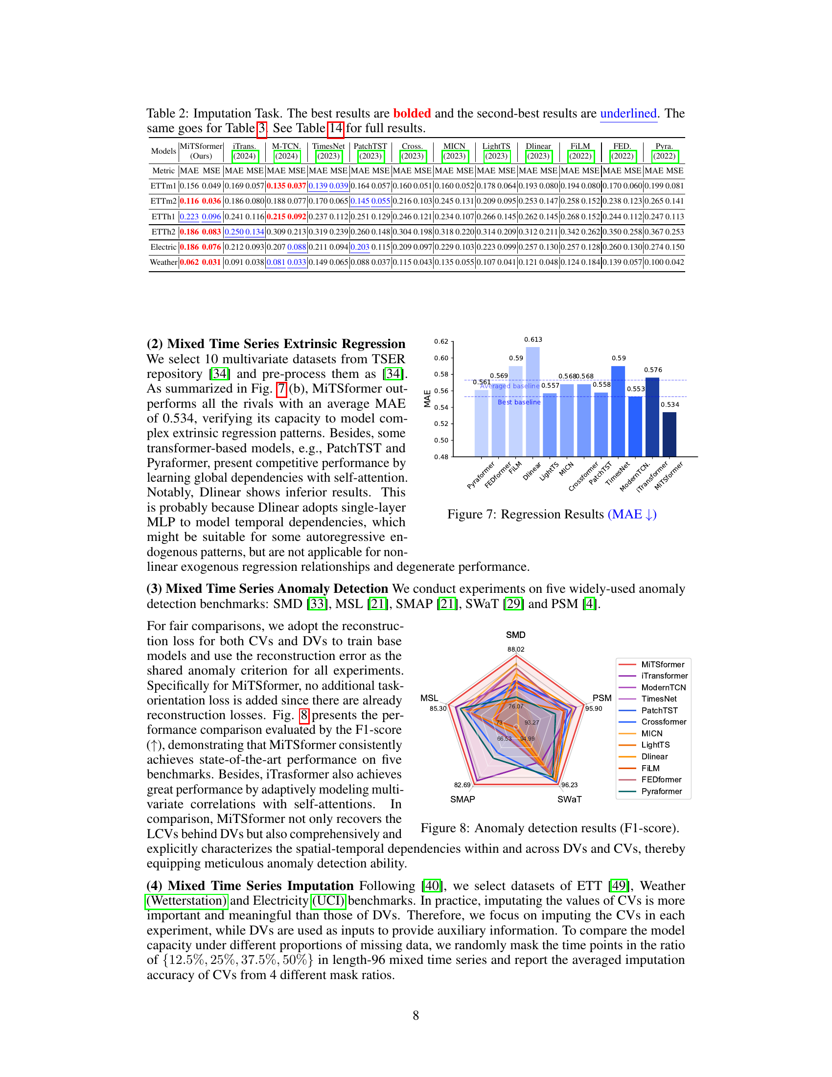
🔼 This radar chart visualizes the F1-scores achieved by MiTSformer and several baseline models on five anomaly detection datasets (SMD, MSL, SMAP, SWaT, and PSM). Each axis represents a dataset, and the radial distance from the center indicates the F1-score for that dataset. Higher values signify better performance. The chart allows for a direct comparison of the models across the different datasets, highlighting MiTSformer’s superior performance in this task.
read the caption
Figure 8: Anomaly detection results (F1-score).

🔼 This figure visualizes the recovery of Latent Continuous Variables (LCVs) from observed Discrete Variables (DVs). Each subplot shows three lines: the observed DVs (blue), the actual LCVs (red), and the recovered LCVs (black). The grey shaded areas highlight time intervals where the observed DVs have a value of 1. The figure demonstrates the MiTSformer’s ability to recover the continuous nature of the underlying variables (LCVs) from their discrete observations (DVs).
read the caption
Figure 9: Visualization of LCV recovery. For each subfigure, the Left plots the observed DVs, and the Right plots the actual LCVs (red line) and recovered LCVs (black line). The grey rectangular patches denotes the area where the observed DV is “1”.

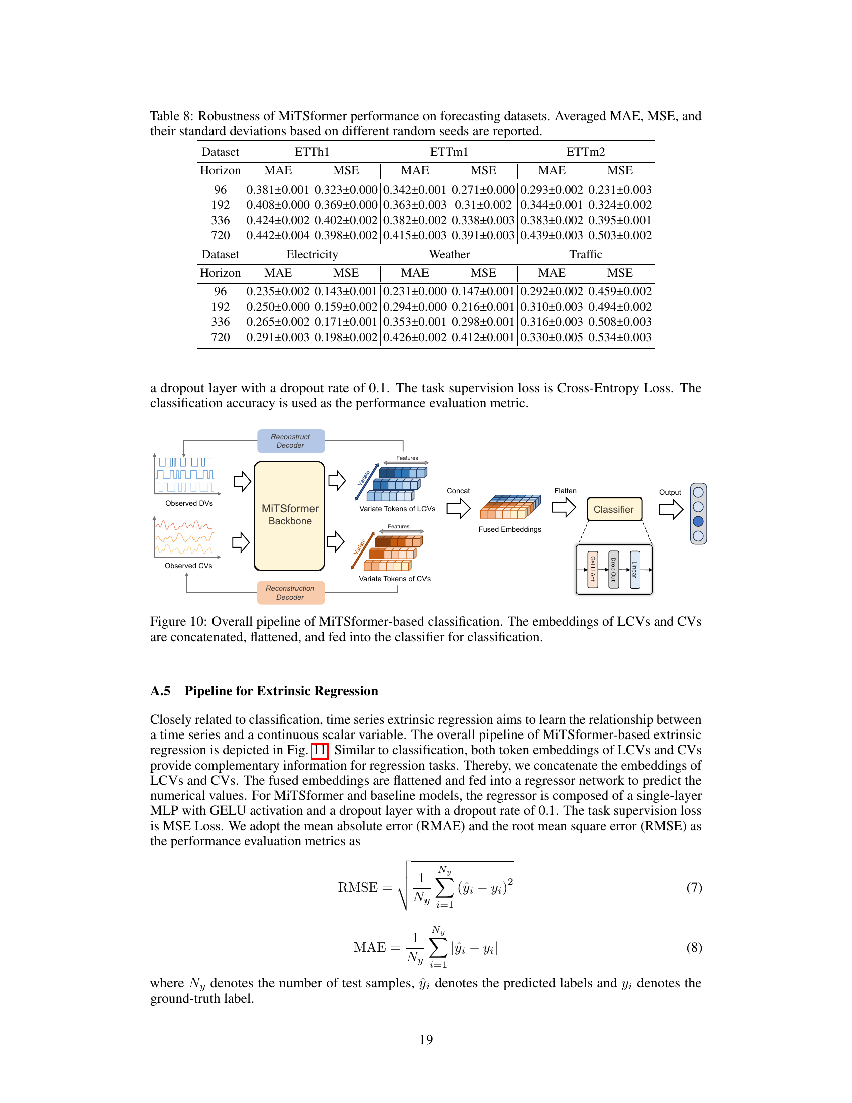
🔼 The figure illustrates the architecture of MiTSformer for the classification task. First, the observed discrete variables (DVs) and continuous variables (CVs) are fed into the MiTSformer backbone. The backbone includes a latent continuity recovery network that recovers latent continuous variables (LCVs) from the DVs and spatial-temporal attention blocks that model dependencies within and across LCVs and CVs. Then, the variate tokens of LCVs and CVs are concatenated and flattened before being fed into a classifier composed of a single-layer MLP with GELU activation and dropout.
read the caption
Figure 10: Overall pipeline of MiTSformer-based classification. The embeddings of LCVs and CVs are concatenated, flattened, and fed into the classifier for classification.

🔼 This figure illustrates the architecture of MiTSformer for the extrinsic regression task. First, observed continuous variables (CVs) and discrete variables (DVs) are input. The DVs are processed by the latent continuity recovery network to obtain latent continuous variables (LCVs). Both LCVs and CVs are then embedded into variate tokens, which capture their respective properties. These tokens are processed by the MiTSformer backbone, which is a combination of self and cross-attention blocks. The resulting fused embeddings are concatenated and flattened before being passed to a regressor to predict the continuous regression output. The regressor itself is a simple multi-layer perceptron (MLP) with GELU activation and dropout regularization.
read the caption
Figure 11: Overall pipeline of MiTSformer-based extrinsic regression. The embeddings of LCVs and CVs are concatenated, flattened, and fed into the regressor for regression.

🔼 The figure shows the overall pipeline of the MiTSformer model. The input is mixed time series data, containing both continuous and discrete variables. The DVs are first processed using latent continuity recovery to obtain latent continuous variables (LCVs). Then, both the LCVs and the original CVs are embedded into variate tokens. These tokens are further processed using spatial-temporal attention blocks, which capture the spatial and temporal dependencies within and across the variables. Finally, the processed tokens are used for two purposes: reconstructing the original time series and performing various downstream analysis tasks. The downstream tasks can include classification, regression, anomaly detection, imputation, and long-term forecasting.
read the caption
Figure 3: Overall pipeline of MiTSformer. First, MiTS undergo latent continuity recovery (DVs only) and are embedded as variate tokens, which are then refined through spatial-temporal attention blocks. The acquired variate tokens are utilized both for reconstructing the original MiTS and serving various downstream tasks.
🔼 This figure illustrates the architecture of MiTSformer, a model designed for mixed time series analysis. It shows the two main stages: 1) Latent Continuity Recovery, focusing on processing discrete variables (DVs) to recover latent continuous variables (LCVs). 2) Spatial-Temporal Attention Blocks, which refine the information from both the LCVs and continuous variables (CVs) using self and cross-attention. The output is used for both reconstructing the original input and performing downstream tasks (e.g., classification, regression).
read the caption
Figure 3: Overall pipeline of MiTSformer. First, MiTS undergo latent continuity recovery (DVs only) and are embedded as variate tokens, which are then refined through spatial-temporal attention blocks. The acquired variate tokens are utilized both for reconstructing the original MiTS and serving various downstream tasks.

🔼 This figure shows the overall architecture of the MiTSformer model. The input is a mixed time series containing both continuous variables (CVs) and discrete variables (DVs). The DVs are first processed by a latent continuity recovery network to recover the underlying continuous variables (LCVs). Both the LCVs and CVs are then embedded as variate tokens. These tokens are passed through spatial-temporal attention blocks to capture the spatial and temporal dependencies within and across the variables. Finally, the refined variate tokens are used for both reconstruction of the original time series and for various downstream tasks such as classification, regression, imputation, and anomaly detection.
read the caption
Figure 3: Overall pipeline of MiTSformer. First, MiTS undergo latent continuity recovery (DVs only) and are embedded as variate tokens, which are then refined through spatial-temporal attention blocks. The acquired variate tokens are utilized both for reconstructing the original MiTS and serving various downstream tasks.
🔼 This figure illustrates the architecture of the spatial-temporal attention blocks within the MiTSformer model. It shows three key components: a variable adjacency matrix that represents relationships between variables, intra-variable self-attention blocks for capturing dependencies within each variable modality (CVs and LCVs), and inter-variable cross-attention blocks that model relationships between the different modalities (CVs and LCVs). The overall design emphasizes capturing complete spatial-temporal dependencies both within and across variable types.
read the caption
Figure 5: Spatial-temporal attention blocks. Left: MiTS variable adjacency matrix, including the variable relationships i) within CVs or LCVs and ii) across CVs and LCVs; Middle: Intra-variable-modality self-attention for modeling spatial-temporal dependencies within CVs or LCVs, and Right: Inter-variable-modality cross-attention for modeling those across CVs and LCVs.
🔼 This figure illustrates the overall architecture of the MiTSformer model. The process begins with latent continuity recovery, focusing solely on the discrete variables (DVs). These DVs are then converted into variate tokens, which serve as inputs to spatial-temporal attention blocks. These blocks refine the tokens by incorporating spatial and temporal dependencies. The output of the attention blocks serves a dual purpose: reconstructing the original mixed time series (MiTS) data and providing inputs for various downstream analysis tasks. This design highlights the model’s ability to handle the heterogeneity of mixed time series and to generate representations suitable for a range of applications.
read the caption
Figure 3: Overall pipeline of MiTSformer. First, MiTS undergo latent continuity recovery (DVs only) and are embedded as variate tokens, which are then refined through spatial-temporal attention blocks. The acquired variate tokens are utilized both for reconstructing the original MiTS and serving various downstream tasks.

🔼 The figure shows the sensitivity analysis of three hyperparameters (λ₁, λ₂, λ₃) in the MiTSformer model. Each subplot shows how classification accuracy changes with different values of one hyperparameter while keeping the others fixed. This demonstrates the impact of each loss component (smoothness, reconstruction, and variable modality discrimination) on the model’s performance for three different classification datasets.
read the caption
Figure 17: Sensitivity analysis of loss items, including smoothness loss weight λ₁, reconstruction loss weight λ₂ and variable modality discrimination loss weight λ₃. Experiments are carried out on classification datasets JapaneseVowels, SpokenArabicDigits, and SelfRegulationSCP1.
More on tables

🔼 This table presents the results for the imputation task, comparing the performance of MiTSformer against several other models on six datasets (ETTm1, ETTm2, ETTh1, ETTh2, Electricity, and Weather). The metrics used to evaluate performance are MAE (Mean Absolute Error) and MSE (Mean Squared Error). The table highlights the best and second-best performing models for each dataset and metric.
read the caption
Table 2: Imputation Task. The best results are bolded and the second-best results are underlined. The same goes for Table 3. See Table 14 for full results.

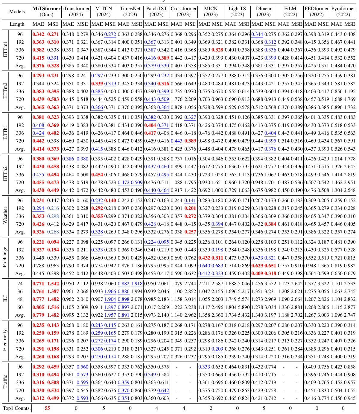
🔼 This table presents the results of long-term forecasting experiments conducted on various datasets. The metrics used are MAE (Mean Absolute Error) and MSE (Mean Squared Error), which are common measures for evaluating the accuracy of forecasting models. The table compares the performance of MiTSformer against several other state-of-the-art models. The ‘-’ indicates that the model ran out of memory for that particular experiment. The full results, including those that ran out of memory, can be found in Table 16.
read the caption
Table 3: Long Term Forecasting of CVs. '-' denotes out of memory. See Table 16 for full results.

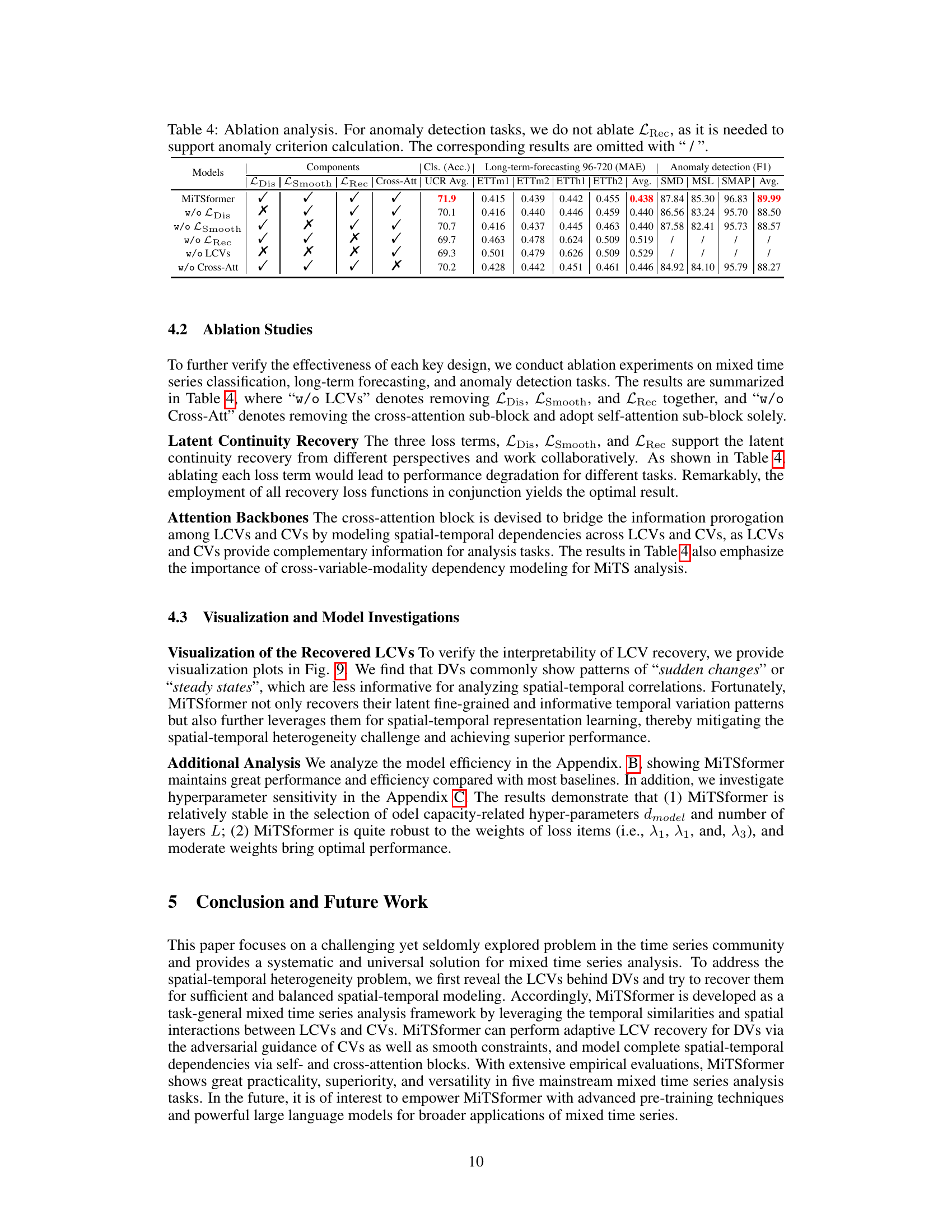
🔼 This ablation study analyzes the impact of each component of MiTSformer on three tasks: classification, long-term forecasting, and anomaly detection. It systematically removes one component at a time (\textit{LDis}, \textit{LSmooth}, \textit{LRec}, Cross-Attention) to observe the effect on performance. The results show that all components are important for optimal performance, particularly the cross-attention mechanism for capturing inter-variable dependencies. Anomaly detection results are not included for the ablation of \textit{LRec} because it is crucial for this task’s anomaly detection criteria.
read the caption
Table 4: Ablation analysis. For anomaly detection tasks, we do not ablate \textit{LRec}, as it is needed to support anomaly criterion calculation. The corresponding results are omitted with ``/\ ''.

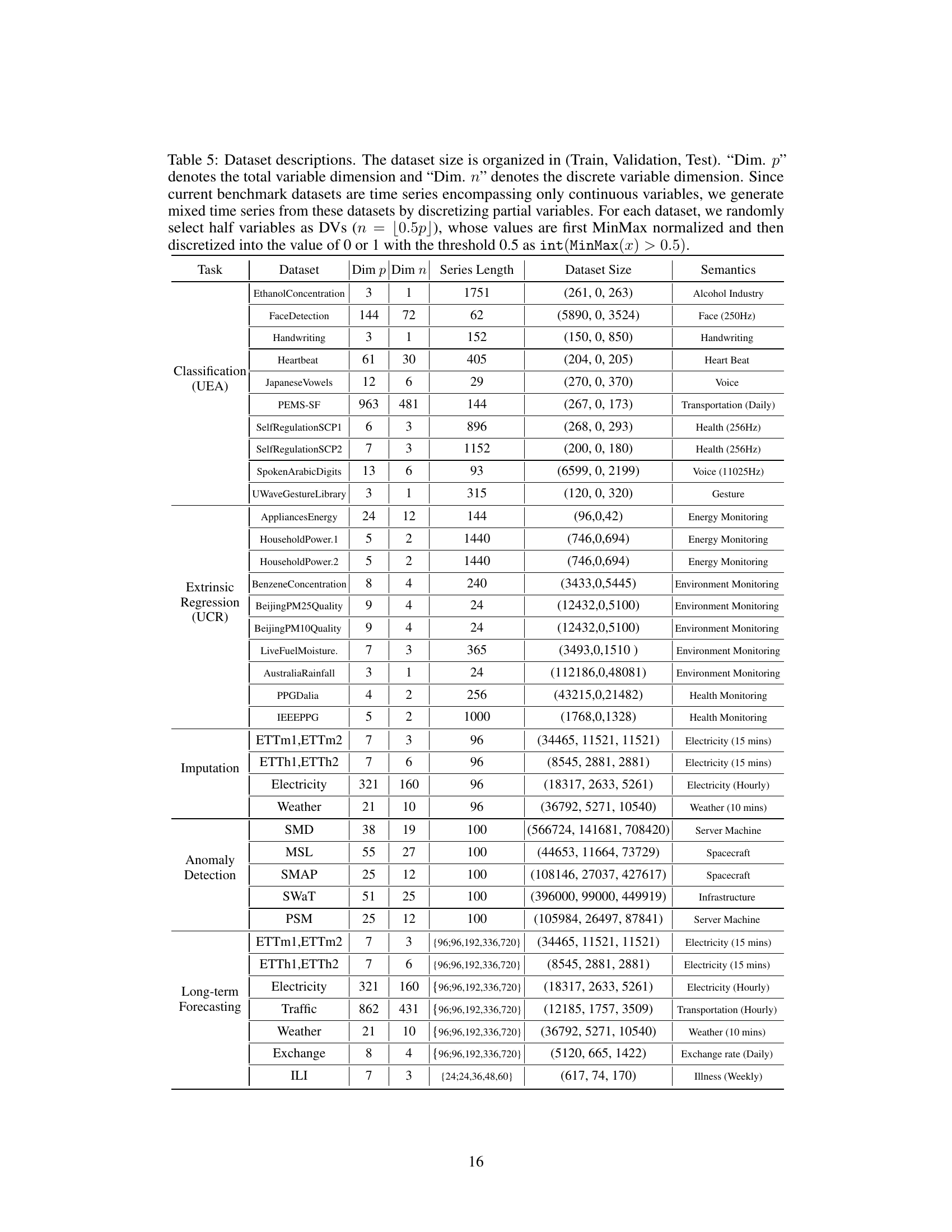
🔼 This table presents the characteristics of the datasets used in the paper’s experiments. It lists each dataset’s name, the number of continuous and discrete variables (Dim p and Dim n respectively), the length of each time series, the size of the dataset split into training, validation, and testing sets, and a short description of the dataset’s content and source. The table highlights how the datasets were adapted to include mixed time series data by converting some continuous variables into discrete variables.
read the caption
Table 5: Dataset descriptions. The dataset size is organized in (Train, Validation, Test). “Dim. p” denotes the total variable dimension and 'Dim. n' denotes the discrete variable dimension. Since current benchmark datasets are time series encompassing only continuous variables, we generate mixed time series from these datasets by discretizing partial variables. For each dataset, we randomly select half variables as DVs (n = [0.5p]), whose values are first MinMax normalized and then discretized into the value of 0 or 1 with the threshold 0.5 as int(MinMax(x) > 0.5).

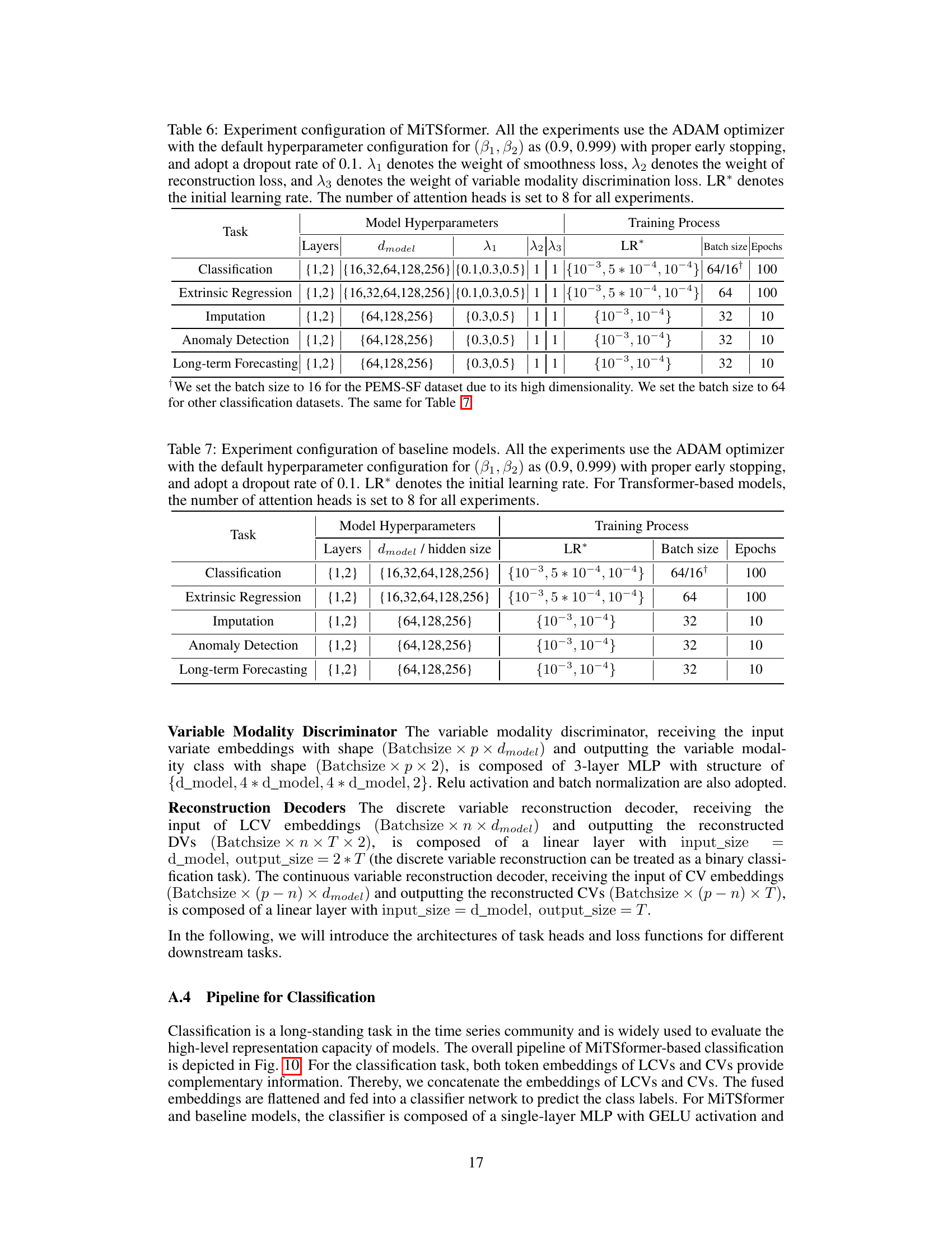
🔼 This table details the hyperparameters used in the MiTSformer model for different tasks. It includes the number of layers, the dimension of the model, the weights assigned to the smoothness, reconstruction, and variable modality discrimination losses, the initial learning rate, batch size, and number of epochs used during training. The ADAM optimizer was used for all experiments with a dropout rate of 0.1 and 8 attention heads.
read the caption
Table 6: Experiment configuration of MiTSformer. All the experiments use the ADAM optimizer with the default hyperparameter configuration for (β1, β2) as (0.9, 0.999) with proper early stopping, and adopt a dropout rate of 0.1. λ₁ denotes the weight of smoothness loss, λ₂ denotes the weight of reconstruction loss, and λ₃ denotes the weight of variable modality discrimination loss. LR* denotes the initial learning rate. The number of attention heads is set to 8 for all experiments.

🔼 This table details the hyperparameter settings used for various baseline models in the experiments. It specifies the optimizer (ADAM), learning rate, batch size, and number of epochs used for training each model on different tasks. The number of attention heads (for transformer-based models) is also specified, along with the layers and hidden size or dmodel dimension.
read the caption
Table 7: Experiment configuration of baseline models. All the experiments use the ADAM optimizer with the default hyperparameter configuration for (β1, β2) as (0.9, 0.999) with proper early stopping, and adopt a dropout rate of 0.1. LR* denotes the initial learning rate. For Transformer-based models, the number of attention heads is set to 8 for all experiments.

🔼 This table demonstrates the robustness of the MiTSformer model’s performance on long-term forecasting tasks across multiple datasets. It shows the average Mean Absolute Error (MAE) and Mean Squared Error (MSE) for four different prediction horizons (96, 192, 336, and 720 time steps), along with the standard deviation for each metric and horizon. The datasets used are ETTm1, ETTm2, ETTh1, ETTh2, Electricity, Weather, and Traffic. This indicates how consistently the model performs across different random initializations of the model parameters, providing a measure of stability and reliability for its forecasting capabilities.
read the caption
Table 8: Robustness of MiTSformer performance on forecasting datasets. Averaged MAE, MSE, and their standard deviations based on different random seeds are reported.

🔼 This table presents a comparison of the classification accuracy achieved by MiTSformer against two other methods: HVM (a mixed Naive Bayes model) and VAMDA (a variational inference-based model). The results show MiTSformer’s superior performance across six different datasets. The table highlights the limitations of the previous methods for this type of mixed-data task, which involve the use of time series data.
read the caption
Table 9: Compared to mixed NB- and VI-based methods. Accuracy(%) scores are reported. The best results are bolded.

🔼 This table presents the results of mixed time series classification experiments conducted with varying numbers of discrete states in the discrete variables (DVs). The accuracy of the classification is reported for each dataset, showing how performance changes as the number of discrete states increases. The best performing model for each dataset is highlighted in bold.
read the caption
Table 10: Performance of mixed time series classification under the different discrete states of DVs, i.e., NDVS. Accuracy (%) scores are reported. The best results are bolded.
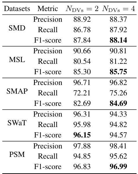
🔼 This table presents the performance of the MiTSformer model and other baseline models on five anomaly detection datasets (SMD, MSL, SMAP, SWAT, PSM). The results are broken down by the number of discrete states (NDVS) in the discrete variables (DVs), comparing results for 2 and 4 discrete states. The metrics reported are Precision, Recall, and F1-score, with higher scores indicating better performance. The best result for each dataset and metric is bolded.
read the caption
Table 11: Performance of mixed time series anomaly detection under the different discrete states of DVs, i.e., NDVs. The best results are bolded.
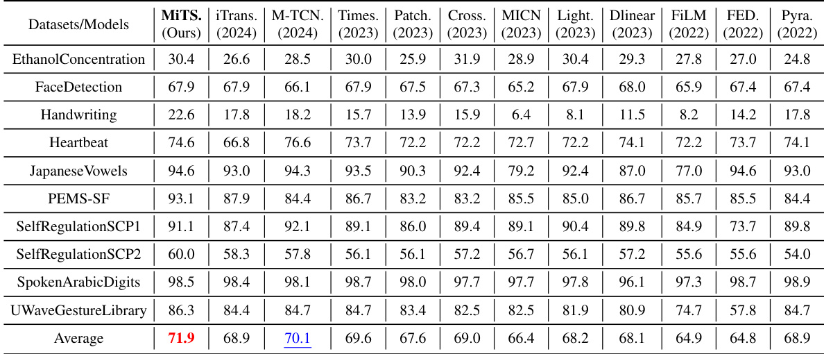
🔼 This table presents the classification accuracy achieved by MiTSformer and various baseline models across ten different datasets. Each dataset represents a distinct time series classification problem, with varying characteristics like length and number of variables. The table allows for a comparison of MiTSformer’s performance against state-of-the-art methods in the context of mixed time series classification. The results highlight MiTSformer’s ability to achieve superior or competitive performance.
read the caption
Table 12: Full classification results. We report the classification accuracy (%) as the result.

🔼 This table demonstrates the robustness of the MiTSformer model’s performance on forecasting tasks across multiple datasets. It shows the average Mean Absolute Error (MAE) and Mean Squared Error (MSE), along with their standard deviations, for different prediction horizons (96, 192, 336, and 720). The results are presented for several datasets: ETTm1, ETTm2, ETTh1, ETTh2, Electricity, Weather, and Traffic, highlighting the model’s consistency and stability across various experimental runs.
read the caption
Table 8: Robustness of MiTSformer performance on forecasting datasets. Averaged MAE, MSE, and their standard deviations based on different random seeds are reported.

🔼 This table presents the robustness analysis of MiTSformer on forecasting tasks. It shows the averaged MAE and MSE values along with their standard deviations across multiple runs (different random seeds) for several datasets and prediction horizons (96, 192, 336, and 720). This demonstrates the stability and reliability of MiTSformer’s performance.
read the caption
Table 8: Robustness of MiTSformer performance on forecasting datasets. Averaged MAE, MSE, and their standard deviations based on different random seeds are reported.

🔼 This table presents the anomaly detection results for five different datasets (SMD, MSL, SMAP, SWAT, and PSM) using MiTSformer and several baseline models. The results are evaluated using precision (P), recall (R), and F1-score (F1), with higher values indicating better performance. The average F1-score across all datasets is also shown for each model.
read the caption
Table 15: Full anomaly detection results. The “P”, “R”, and “F1” represent the precision, recall, and F1-score (%) respectively. F1-score is the harmonic mean of precision and recall. A higher value of P, R, and F1 indicates better anomaly detection performance.
🔼 This table demonstrates the robustness of the MiTSformer model’s performance on long-term forecasting tasks across multiple datasets. It presents the average Mean Absolute Error (MAE) and Mean Squared Error (MSE), along with their standard deviations, calculated from multiple runs with different random seeds. This helps assess the stability and reliability of the model’s predictions across various runs.
read the caption
Table 8: Robustness of MiTSformer performance on forecasting datasets. Averaged MAE, MSE, and their standard deviations based on different random seeds are reported.

🔼 This table presents the robustness analysis of MiTSformer’s performance on long-term forecasting tasks. It shows the average Mean Absolute Error (MAE) and Mean Squared Error (MSE), along with their standard deviations, calculated across multiple runs with different random seeds. The results are reported for different forecasting horizons (96, 192, 336, and 720) on several datasets (ETTm1, ETTm2, ETTh1, ETTh2, Electricity, Weather, and Traffic). This demonstrates the stability and reliability of MiTSformer’s performance across various runs.
read the caption
Table 8: Robustness of MiTSformer performance on forecasting datasets. Averaged MAE, MSE, and their standard deviations based on different random seeds are reported.
Full paper#

