TL;DR#
Many machine learning algorithms rely on computationally expensive matrix-vector multiplications, especially when dealing with large graphs. Existing methods often struggle with the speed and scalability required for real-world applications. This paper tackles this challenge by focusing on integrating tensor fields on trees, a simplified but relevant structure for many graph-based tasks.
The researchers introduce novel algorithms called Fast Tree-Field Integrators (FTFIs). These algorithms cleverly leverage the structure of trees to drastically reduce the computation time for these integrations. Importantly, FTFIs are highly efficient and, in many cases, provide exact solutions. Experiments show significant speed improvements (5.7-13x) when compared to brute-force methods, along with accuracy gains of 1.0-1.5% in certain applications. The results suggest that FTFIs can greatly accelerate various graph-based machine learning tasks.
Key Takeaways#
Why does it matter?#
This paper is crucial for researchers working with large-scale graphs and neural networks. It offers significantly faster algorithms for common graph operations, impacting fields like machine learning and computer vision. The introduction of learnable parameters within the proposed framework opens exciting avenues for further research and optimization, particularly regarding topological transformers and vision applications.
Visual Insights#
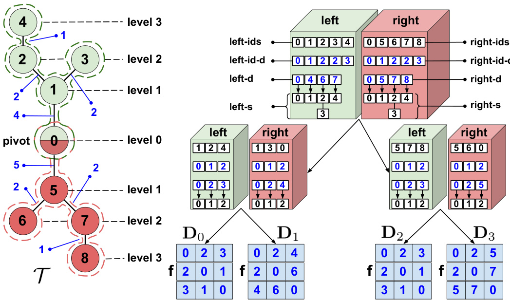
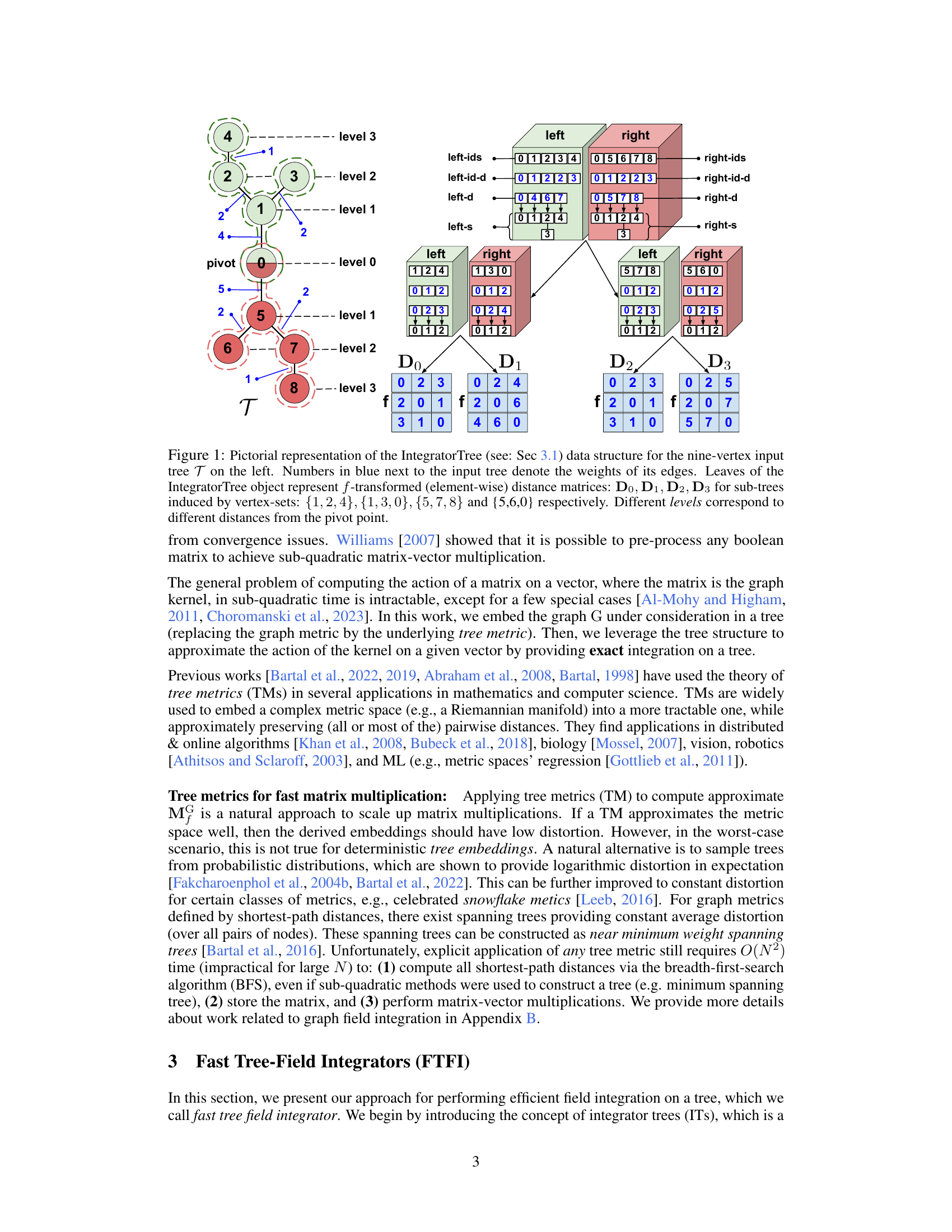
🔼 This figure illustrates the IntegratorTree data structure, a key component of the Fast Tree-Field Integrators (FTFIs) algorithm. The IntegratorTree is a binary tree that recursively decomposes the input tree (T) into smaller subtrees. Each leaf node of the IntegratorTree represents an f-transformed distance matrix for its corresponding subtree, where f is a function applied element-wise to the distance matrix. The non-leaf nodes store information to efficiently navigate and compute the integration across subtrees. The diagram shows how the tree is decomposed, highlighting pivot points and the resulting distance matrices at the leaf nodes.
read the caption
Figure 1: Pictorial representation of the IntegratorTree (see: Sec 3.1) data structure for the nine-vertex input tree T on the left. Numbers in blue next to the input tree denote the weights of its edges. Leaves of the IntegratorTree object represent f-transformed (element-wise) distance matrices: D0, D1, D2, D3 for sub-trees induced by vertex-sets: {1, 2, 4}, {1,3, 0}, {5, 7,8} and {5,6,0} respectively. Different levels correspond to different distances from the pivot point.

🔼 This table shows the performance of different Topological Vision Transformer models using tree-based masking. Each row represents a different configuration of the model, specifying the activation function used, whether parameter sharing was used across different attention heads (synced), and the number of extra learnable parameters per layer. The table compares the accuracy of these models on the ImageNet and Places365 datasets. The best-performing model for each configuration is highlighted in bold, and the results for the Performer baselines are shown in blue.
read the caption
Table 1: Performance of Topological Vision Transformers with tree-based masking. For each attention kernel, we present the results of the best variant in bold and Performer baselines in blue.
In-depth insights#
Tree-Field Int.#
The heading ‘Tree-Field Int.’ likely refers to a novel method for integrating tensor fields defined on tree structures. This suggests a computationally efficient algorithm leveraging the inherent hierarchical nature of trees for faster processing compared to general graph-based methods. The approach likely involves a divide-and-conquer strategy, recursively processing subtrees and combining results efficiently. This efficiency could be achieved through smart data structures like balanced binary trees or other specialized tree decompositions to minimize computational complexity and storage requirements. The “Tree-Field” aspect implies that the method works directly on tree representations of data, rather than requiring explicit matrix representations. Exactness is a possible key feature, meaning the integration provides numerically identical results to brute-force calculation, but dramatically faster. The theoretical analysis of the method would likely focus on proving its computational complexity bounds, likely showing polylogarithmic or near-linear time complexity depending on the specifics of the implementation. Applications are key, and likely involve scenarios where data can be naturally represented as trees or efficiently approximated by them, such as hierarchical data, branching processes, and various ML tasks.
FTFI Efficiency#
The efficiency of Fast Tree-Field Integrators (FTFIs) is a central theme, showcasing significant speedups over traditional methods. Exact FTFIs achieve 5.7-13x speed improvements when applied to large graphs (thousands of nodes), demonstrating their practical advantage. This is primarily due to the algorithm’s polylog-linear time complexity, a substantial improvement over the brute-force quadratic time of baseline methods. The speed advantage is consistent across different graph types, such as synthetic graphs and meshes from real-world datasets. The approximation quality of FTFIs is also considered, with experiments showing competitive performance compared to other approximation techniques. Although approximation quality is affected by the choice of tree metric used, the efficiency gains remain substantial, suggesting that FTFIs are a powerful tool for large-scale graph processing.
Appx. Quality#
The heading ‘Appx. Quality’ suggests an appendix section dedicated to evaluating the quality of an approximation method. This likely involves a detailed analysis of the approximation’s accuracy, efficiency, and robustness. Key aspects might include a comparison of the approximation against a ground truth or a more accurate, but computationally expensive, method. The appendix could present quantitative results, such as error metrics and runtime comparisons under varying conditions. It could also include qualitative assessments, such as visualizations or subjective evaluations of the quality of the output. The level of detail in ‘Appx. Quality’ would depend on the specific approximation method and its intended application. A focus on practical considerations, such as the trade-off between accuracy and computational cost, is probable. It would be beneficial if it included considerations of how the approximation’s quality scales with problem size and whether it’s suitable for large-scale applications. Finally, the reliability of the approximation and its sensitivity to noise or other factors would be significant considerations within the ‘Appx. Quality’ assessment.
Learnable F-Dist#
The heading ‘Learnable F-Dist’ suggests a research focus on learning the parameters of a distance function, denoted as ‘f’, within a specific context. This implies a departure from using pre-defined or fixed distance metrics, and instead, adapting the function ‘f’ based on data. This approach is likely motivated by improving the accuracy or efficiency of algorithms that rely on such distances. The ‘Learnable F-Dist’ concept would entail defining a parameterized family of distance functions (e.g., using neural networks), and then training this model to learn the optimal parameters given specific input data or tasks. This learning process could leverage supervised, unsupervised, or reinforcement learning paradigms. The key advantages expected are improved accuracy through better adaptation to the data’s underlying structure, and increased efficiency by potentially simplifying computation. However, challenges include careful design of the parameterized family, preventing overfitting, and ensuring the learned function remains a valid distance metric (satisfying properties such as non-negativity, identity of indiscernibles, symmetry, and the triangle inequality).
TopViT Ext.#
The heading ‘TopViT Ext.’ suggests an extension or enhancement to a pre-existing model called TopViT, likely a type of vision transformer. This extension probably involves improving TopViT’s capabilities, possibly by integrating new techniques or addressing limitations. The extension might focus on enhancing efficiency, accuracy, or scalability of the original TopViT architecture. This could involve modifications to the attention mechanism, positional encoding, or other key components, perhaps integrating novel methods for faster computations or improved representation learning. The ‘Ext’ likely implies a novel approach rather than merely a parameter tuning exercise. Specific details would depend on the paper’s content. It is probable that the ‘Ext’ version of TopViT would be evaluated and compared against the original TopViT to demonstrate its improvements. The experiments would quantify the performance gains in various aspects, possibly reporting metrics such as accuracy, computational cost, and memory usage.
More visual insights#
More on figures

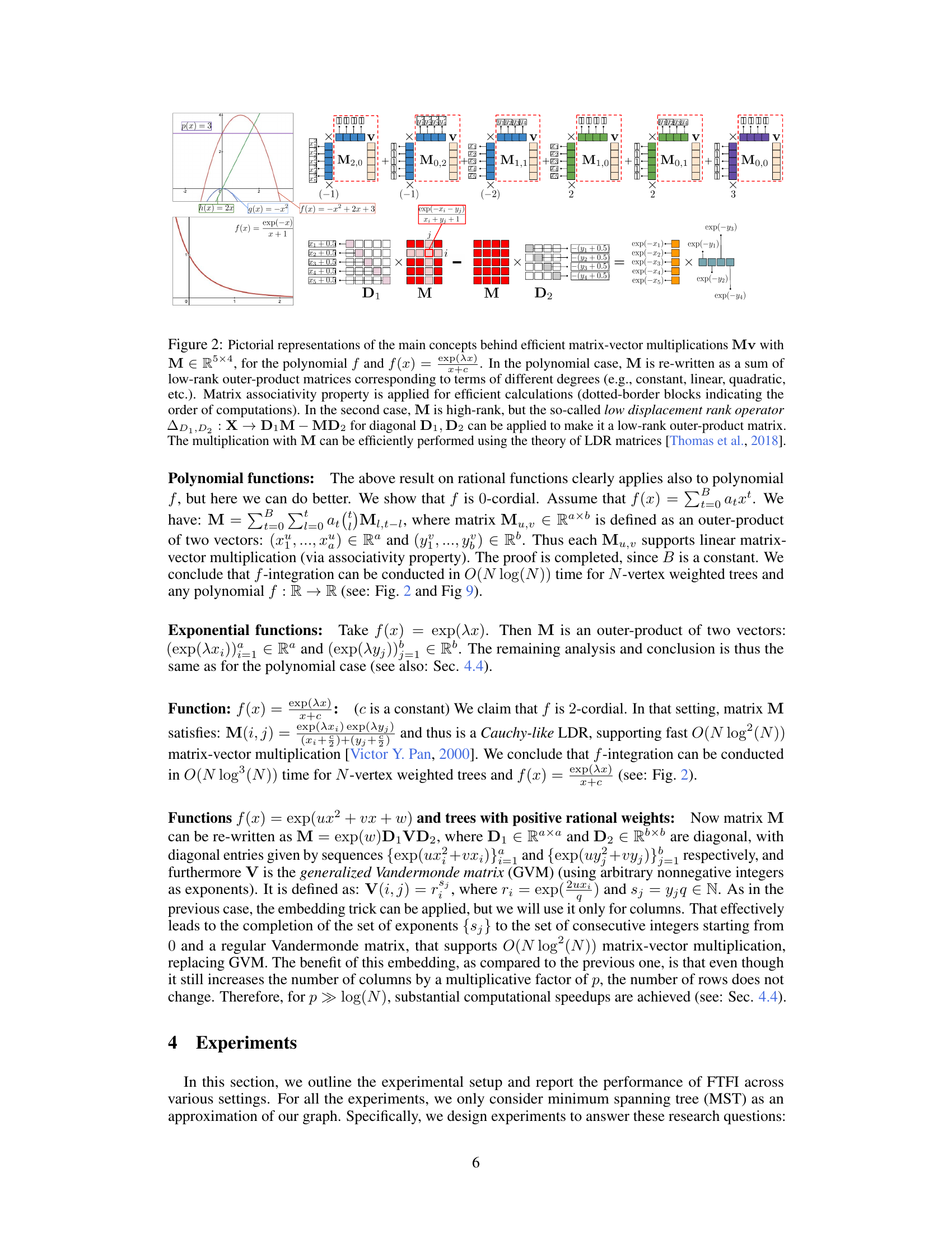
🔼 This figure demonstrates how matrix-vector multiplications can be made efficient using low displacement rank matrices. It shows two examples, one for polynomial functions and another for exponential functions. The polynomial case uses a sum of low-rank outer product matrices, and the exponential case uses a low displacement rank operator to reduce the rank of the matrix.
read the caption
Figure 2: Pictorial representations of the main concepts behind efficient matrix-vector multiplications Mv with M∈ R5×4, for the polynomial f and f(x) = exp(x). In the polynomial case, M is re-written as a sum of low-rank outer-product matrices corresponding to terms of different degrees (e.g., constant, linear, quadratic, etc.). Matrix associativity property is applied for efficient calculations (dotted-border blocks indicating the order of computations). In the second case, M is high-rank, but the so-called low displacement rank operator AD1,D2: X → D1M – MD2 for diagonal D1, D2 can be applied to make it a low-rank outer-product matrix. The multiplication with M can be efficiently performed using the theory of LDR matrices [Thomas et al., 2018].

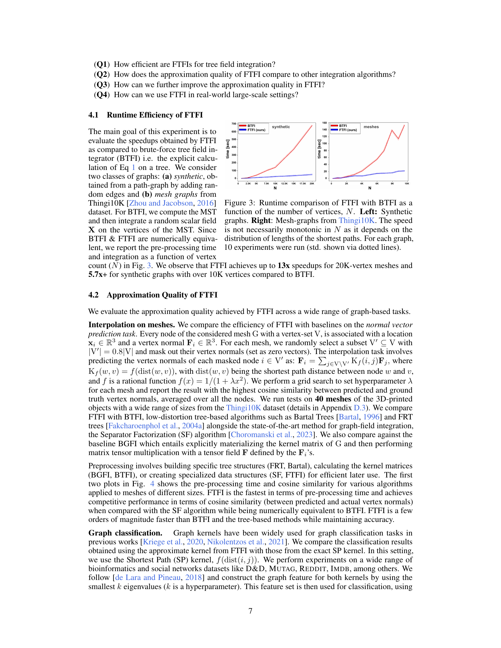
🔼 This figure compares the runtime performance of the proposed Fast Tree-Field Integrators (FTFI) algorithm against a brute-force baseline (BTFI) for tree field integration. The comparison is shown for two types of graphs: synthetic graphs and mesh graphs from the Thingi10K dataset. The x-axis represents the number of vertices (N) in the graph, and the y-axis represents the runtime in seconds. The results show that FTFI is significantly faster than BTFI, especially for larger graphs, achieving speedups of up to 13x for mesh graphs and 5.7x for synthetic graphs. Error bars representing standard deviation across 10 runs are included.
read the caption
Figure 3: Runtime comparison of FTFI with BTFI as a function of the number of vertices, N. Left: Synthetic graphs. Right: Mesh-graphs from Thingi10K. The speed is not necessarily monotonic in N as it depends on the distribution of lengths of the shortest paths. For each graph, 10 experiments were run (std. shown via dotted lines).

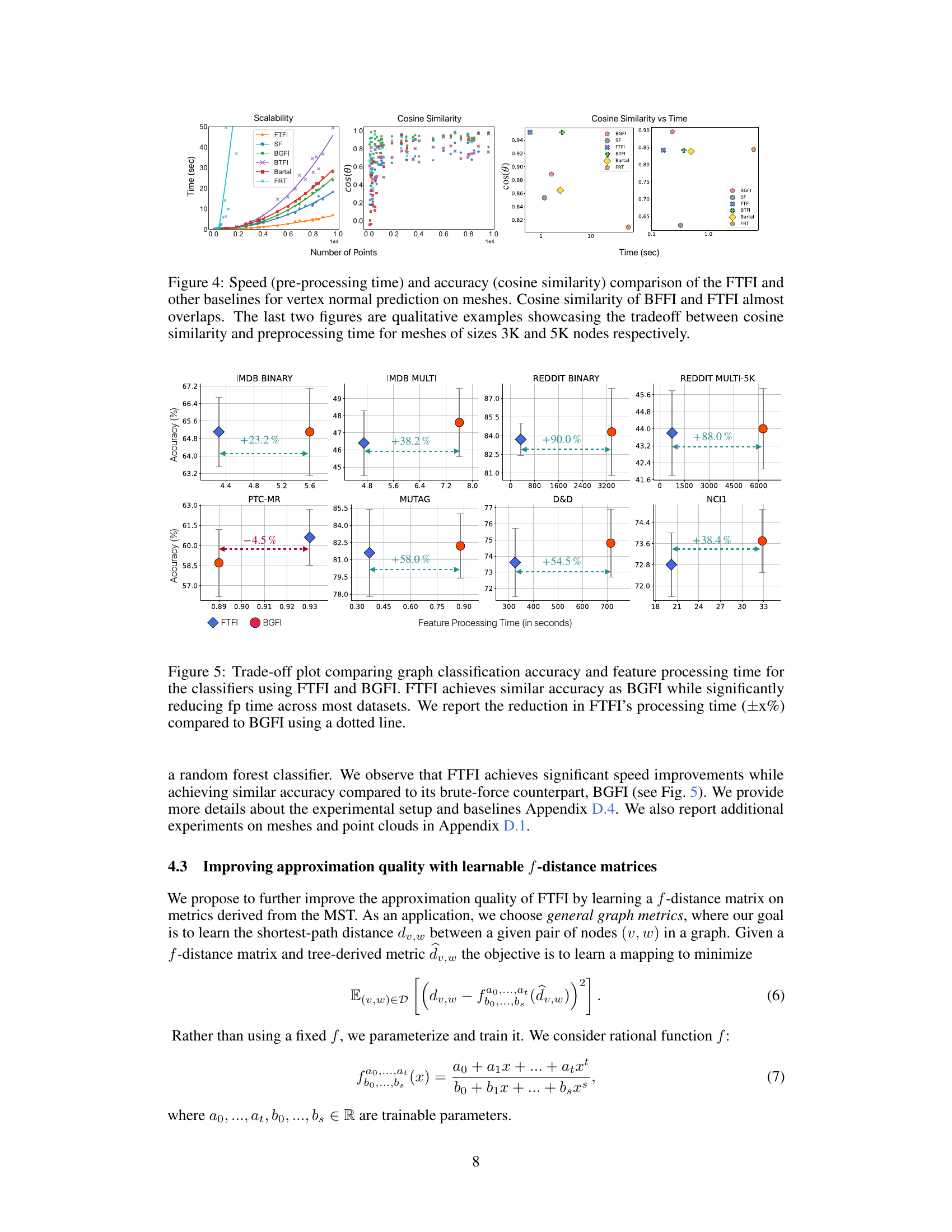
🔼 This figure compares the performance of FTFI against other methods for vertex normal prediction on meshes from the Thingi10K dataset. It shows that FTFI is much faster (pre-processing time) than other methods while maintaining comparable accuracy (cosine similarity). The plots illustrate the trade-off between pre-processing time and accuracy for different mesh sizes (3K and 5K nodes).
read the caption
Figure 4: Speed (pre-processing time) and accuracy (cosine similarity) comparison of the FTFI and other baselines for vertex normal prediction on meshes. Cosine similarity of BFFI and FTFI almost overlaps. The last two figures are qualitative examples showcasing the tradeoff between cosine similarity and preprocessing time for meshes of sizes 3K and 5K nodes respectively.
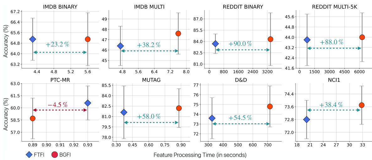
🔼 This figure shows a comparison of the trade-off between graph classification accuracy and feature processing time for FTFI and BGFI across multiple datasets. It demonstrates that FTFI achieves comparable accuracy to BGFI while significantly reducing feature processing time.
read the caption
Figure 5: Trade-off plot comparing graph classification accuracy and feature processing time for the classifiers using FTFI and BGFI. FTFI achieves similar accuracy as BGFI while significantly reducing fp time across most datasets. We report the reduction in FTFI's processing time (±x%) compared to BGFI using a dotted line.

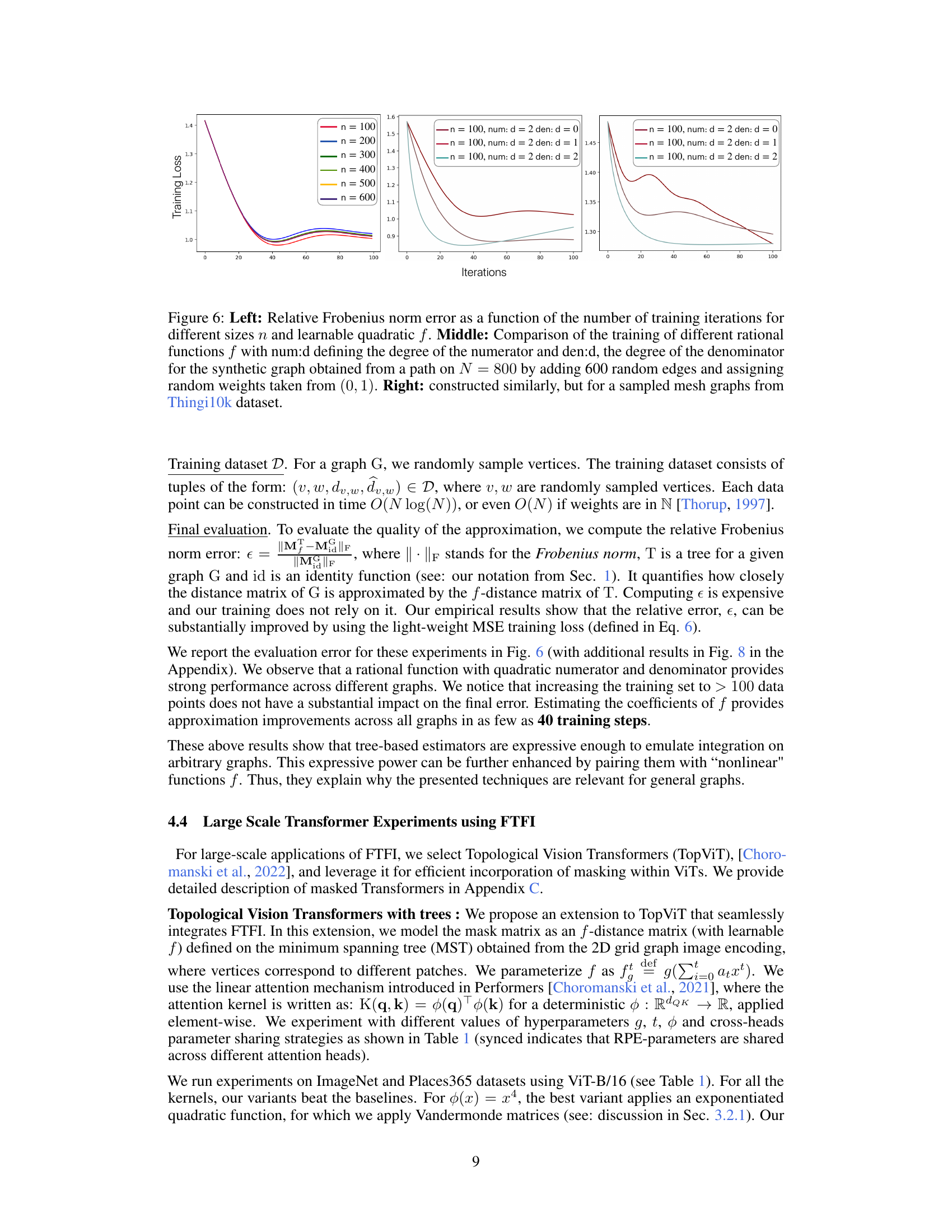
🔼 The figure shows the results of training learnable f-distance matrices using different rational functions with varying degrees of numerator and denominator. The left panel displays the relative Frobenius norm error for different graph sizes, while the middle and right panels compare the training curves for synthetic and mesh graphs, respectively.
read the caption
Figure 6: Left: Relative Frobenius norm error as a function of the number of training iterations for different sizes n and learnable quadratic f. Middle: Comparison of the training of different rational functions f with num:d defining the degree of the numerator and den:d, the degree of the denominator for the synthetic graph obtained from a path on N = 800 by adding 600 random edges and assigning random weights taken from (0, 1). Right: constructed similarly, but for a sampled mesh graphs from Thingi10k dataset.
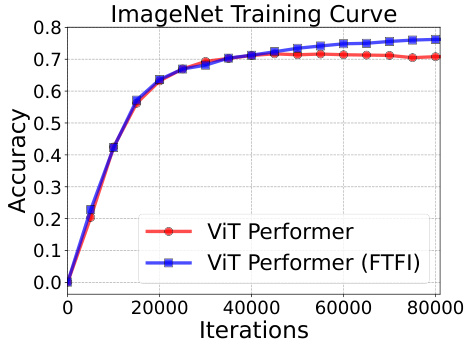
🔼 This figure shows the training accuracy curves for the ViT Performer model and the ViT Performer model with FTFI on the ImageNet dataset. The FTFI-augmented model shows a significantly higher accuracy than the baseline Performer model, demonstrating a 7% improvement.
read the caption
Figure 7: Left: Experiments with the RPE mechanism for ViT-B and on ImageNet. We observe that FTFI provides 7% accuracy gain compared to the Performer variant.

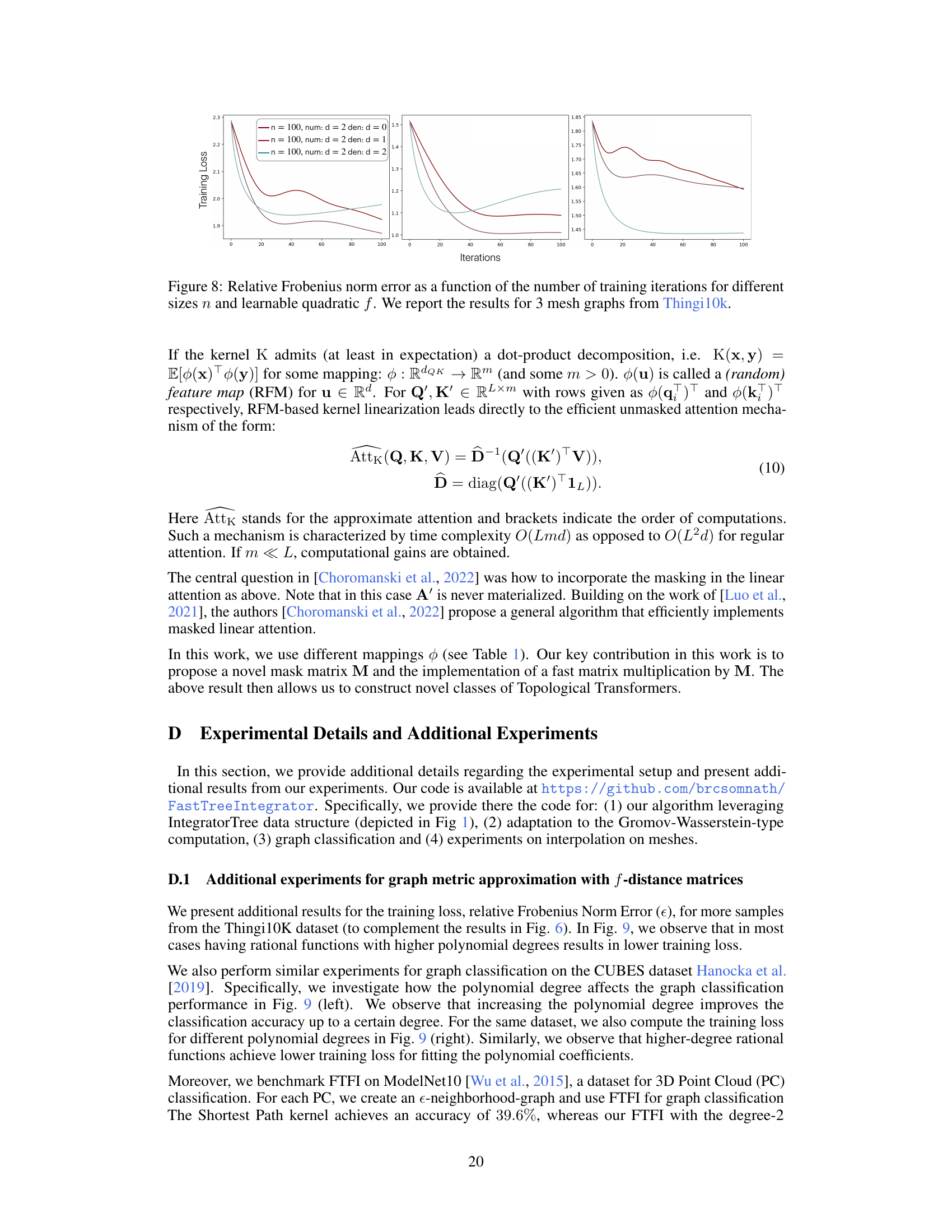
🔼 The figure shows the relative Frobenius norm error for different sizes of synthetic graphs (n = 100, 200, 300, 400, 500, 600) and different rational functions (num:d=2, den:d=0, 1, 2). The training loss is plotted against the number of iterations. Each subplot shows results for a different mesh graph from the Thingi10k dataset.
read the caption
Figure 8: Relative Frobenius norm error as a function of the number of training iterations for different sizes n and learnable quadratic f. We report the results for 3 mesh graphs from Thingi10k.
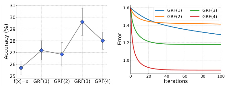
🔼 The left plot shows the accuracy of graph classification on the CUBES dataset for different rational functions (GRF). The degree of the GRF polynomials is varied from 1 to 4. The right plot shows the training loss curves for learning the coefficients of those same rational functions; the plot indicates that using higher degree rational functions leads to lower training loss.
read the caption
Figure 9: Left: Variation in FTFI performance with different f-distance functions on the CUBES dataset. We use general rational functions (GRF) of varying polynomial degrees. GRF(i) indicates a rational function of the i-th degree. We observe a general trend of accuracy increase with function complexity up to a certain degree. The coefficients of the GRF were learnt using a few graph instances. Right: We show the training loss curves for estimating the coefficients of the rational function, f, for samples in the CUBES dataset. We report the training loss for rational functions with varying polynomial degrees. We observe that the training loss is lower when we use rational functions with high-degree polynomials.
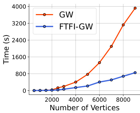
🔼 The figure compares the computation time of Gromov-Wasserstein (GW) distance calculation against the proposed Fast Tree-Field Integrator (FTFI) enhanced GW approach. The x-axis represents the number of vertices in the graph, and the y-axis shows the computation time in seconds. The results demonstrate that FTFI-GW significantly reduces the computation time compared to the standard GW method, especially as the number of vertices increases.
read the caption
Figure 10: Comparison of field integration time between GW and FTFI-GW. We observe that FTFI achieves significant computation time gain over the baseline.
More on tables
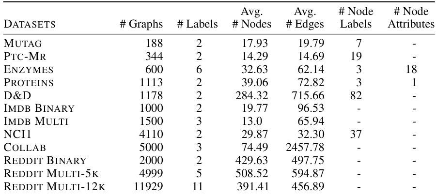
🔼 This table presents the characteristics of various graph datasets employed for graph classification in the research paper. For each dataset, it lists the number of graphs, the number of classes (labels), the average number of nodes per graph, the average number of edges per graph, the number of node labels (if any), and the number of node attributes (if any). This information is crucial for understanding the scale and complexity of the datasets used in the experiments and for evaluating the generalizability of the results.
read the caption
Table 2: Statistics of the graph classification datasets used in this paper.
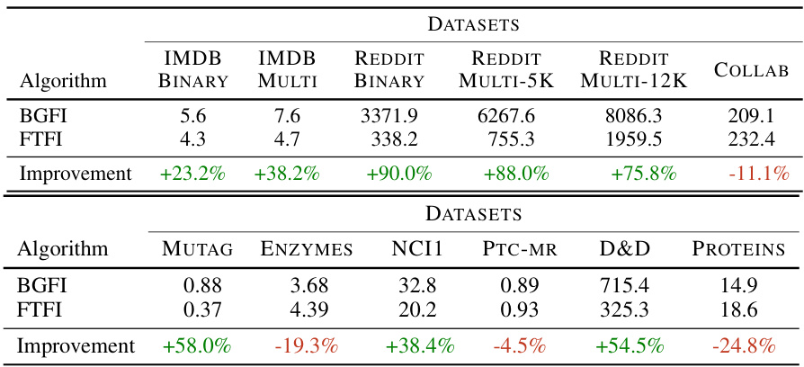
🔼 This table compares the time taken for feature processing using the Fast Tree-Field Integrator (FTFI) method against the exact shortest path kernel computation (BGFI). It shows the processing time for various graph datasets (MUTAG, ENZYMES, NCI1, PTC-MR, D&D, PROTEINS) and highlights the significant speedup achieved by FTFI in most cases, with reductions up to 90%.
read the caption
Table 3: Feature processing time of FTFI compared to exact shortest path kernel computation. We observe that FTFI achieves significant speedups up to 90% reduction in processing time. All times are reported in seconds (s).
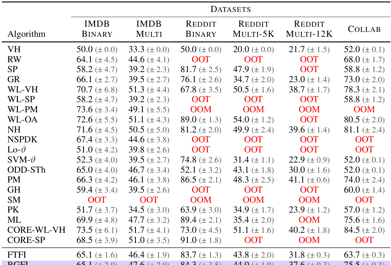
🔼 This table compares the performance of the Fast Tree-Field Integrator (FTFI) algorithm against various baseline graph kernel classification methods on several datasets. It demonstrates that FTFI achieves comparable accuracy to the exact shortest path (SP) kernel, while offering significant speed improvements over other methods.
read the caption
Table 4: Comparison of FTFI with a broad range of graph kernel-based classification approaches. We observe that FTFI achieves performance similar to that of Exact SP, its exact counterpart, across almost all datasets. The baseline results have been compiled from Nikolentzos et al. [2021]. OOT and OOM indicate that the corresponding algorithm ran out of time or memory respectively.
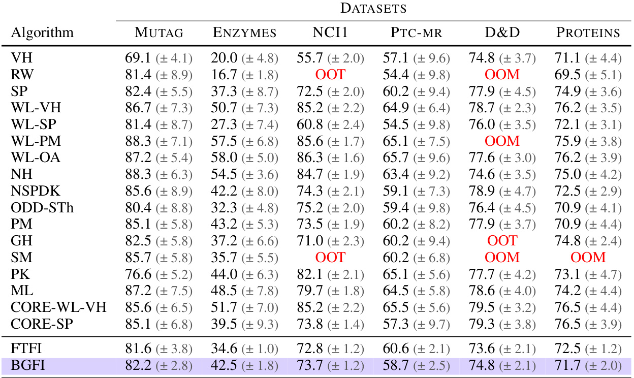
🔼 This table compares the performance of the proposed Fast Tree-Field Integrator (FTFI) method against various existing graph kernel-based classification approaches across multiple datasets. It shows that FTFI achieves comparable accuracy to the exact Shortest Path (SP) kernel method, which it is designed to approximate, while significantly outperforming many other techniques. Note that ‘OOT’ signifies that the algorithm ran out of time, and ‘OOM’ means it ran out of memory. The baseline results are taken from a previous publication by Nikolentzos et al. (2021).
read the caption
Table 4: Comparison of FTFI with a broad range of graph kernel-based classification approaches. We observe that FTFI achieves performance similar to that of Exact SP, its exact counterpart, across almost all datasets. The baseline results have been compiled from Nikolentzos et al. [2021]. OOT and OOM indicate that the corresponding algorithm ran out of time or memory respectively.

🔼 This table presents the hyperparameters used for the various Vision Transformer (ViT) models in the experiments. It shows the number of heads, layers, hidden dimension, MLP dimension, total number of parameters, and patch size for ViT-Base and ViT-Large (16). These settings are crucial for understanding the computational cost and performance of the different models.
read the caption
Table 5: Hyperparameters for the different ViT models used in this paper
🔼 This table presents the performance of different Topological Vision Transformer models on ImageNet and Places365 datasets. The models use tree-based masking, and for each attention kernel, the table shows the accuracy achieved by the best performing model variant. It also includes results for Performer baselines for comparison.
read the caption
Table 1: Performance of Topological Vision Transformers with tree-based masking. For each attention kernel, we present the results of the best variant in bold and Performer baselines in blue.
Full paper#
