TL;DR#
Many real-world systems are modeled using linear causal models, but often only a subset of variables is observable. Existing methods for parameter identification are limited as they typically focus on the edges between observed variables, ignoring the relationships involving latent (unobserved) variables. This leads to issues in accurately recovering causal effects and making reliable predictions.
This research proposes a more general framework that addresses these limitations. They introduce graphical conditions to determine when model parameters are identifiable, considering the flexible relationships between observed and latent variables. They also present a new likelihood-based estimation method that effectively handles various types of indeterminacy in parameter estimation. Their empirical results using both simulated and real-world datasets validate their theoretical findings and demonstrate the effectiveness of their method in recovering model parameters accurately.
Key Takeaways#
Why does it matter?#
This paper is crucial for researchers working with partially observed linear causal models. It offers novel theoretical insights into parameter identifiability, addressing limitations of existing methods. The proposed likelihood-based estimation method is readily applicable to real-world problems and opens avenues for more accurate causal inference in complex systems.
Visual Insights#

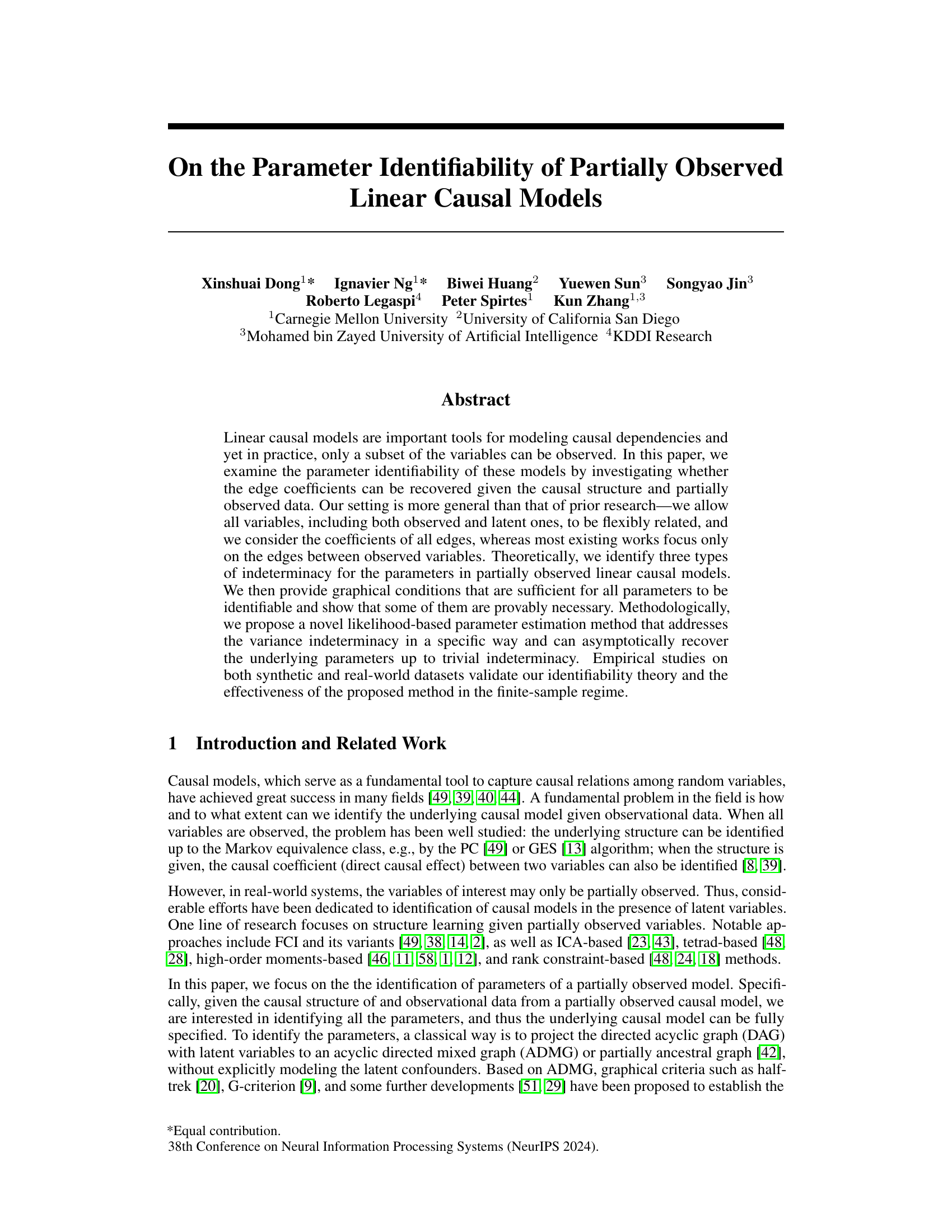
🔼 This figure compares two different causal graphs (G1 and G2) and their corresponding ADMG (acyclic directed mixed graph) representation after projecting out latent variables. G1’s parameters are identifiable in the proposed framework, while G2’s are not. The latent projection framework, however, fails to distinguish between G1 and G2 because they share the same ADMG. This highlights the advantage of the proposed framework which considers all variables and edges, unlike the latent projection method which only considers observed variables and loses information about latent variable connections.
read the caption
Figure 1: Illustrations of the advantage of our framework. Within our framework, it can be shown that G₁'s parameters can be identified (up to sign) while G2's cannot. In contrast, the latent projection framework cannot even differentiate G₁ from G2 as they share the same ADMG (c) after projection. Furthermore, with ADMG, any edge coefficient that involves a latent variable cannot be considered.

🔼 This table presents the mean and standard deviation of the Mean Squared Error (MSE) for two different parameter estimation methods (Estimator and Estimator-TR) applied to synthetic datasets. The MSE is calculated for two scenarios: up to group sign indeterminacy (GS Case) and up to orthogonal transformation indeterminacy (OT Case). The results are shown for three different sample sizes (2k, 5k, and 10k) to demonstrate the performance of the methods across varying data amounts.
read the caption
Table 1: Experimental result on synthetic data using MSE (mean (std)).
In-depth insights#
Partial ID Theory#
A hypothetical ‘Partial ID Theory’ in a research paper would likely explore the identifiability of parameters in a system where only partial information is available. This could involve scenarios with latent variables, missing data, or limited observability. The core of the theory would likely center on establishing conditions under which it’s possible to uniquely determine the parameters despite the incomplete data. Sufficient conditions would specify sets of assumptions or constraints that, if met, guarantee identifiability. Conversely, necessary conditions would identify minimal requirements for identifiability, highlighting the limits of what can be achieved with partial information. The theory might also examine the types of indeterminacy that arise when identifiability isn’t guaranteed—for example, cases where multiple parameter sets could explain the observed data equally well. A robust partial ID theory would ideally provide both graphical criteria (using causal diagrams) and algebraic conditions to assess identifiability, offering a comprehensive framework for analyzing systems with incomplete information. The practical applications could be far-reaching, impacting fields relying on causal inference with potentially incomplete data.
Graphical Conditions#
The section on “Graphical Conditions” likely details the visual representation of causal relationships within a model, using graphs to represent variables and their connections. It probably explores how the structure of these graphs – including the presence of directed and bidirected edges, cycles, and the arrangement of observed and latent variables – impacts the identifiability of model parameters. The authors likely present sufficient graphical conditions that, if met, guarantee the unique determination of parameters up to some inherent indeterminacies. These conditions may involve the absence of certain graph structures, or the presence of specific patterns. The conditions would be crucial in assessing whether observed data is enough to uniquely estimate the causal effects encoded within the model. A key aspect would be distinguishing between identifiable and non-identifiable scenarios and how the graph’s structure determines whether causal parameters can be uniquely recovered from the data. Sufficiency is important; while necessary conditions might exist, the provided conditions probably aim to be sufficient, ensuring that if the conditions hold true, identifiability is assured. The use of graphical criteria allows researchers to visually assess the identifiability of their model before attempting parameter estimation, greatly improving the efficiency and reliability of causal analysis.
Parameter Estimation#
The parameter estimation section of a research paper is crucial as it bridges the theoretical framework with practical application. It details the methodology used to estimate model parameters using observed data. A robust method is essential, demonstrating its ability to handle various data characteristics and limitations. The description should clearly outline the estimation technique employed, such as maximum likelihood estimation, Bayesian methods, or other statistical approaches. Key implementation details are critical for reproducibility: specifying parameterizations, optimization algorithms used (e.g., gradient descent, Expectation-Maximization), and handling of constraints or regularization techniques. Crucially, the section should address potential challenges in parameter identification such as the presence of latent variables or model misspecifications. Assessing the performance is vital, often done through metrics like mean squared error, bias, and variance, ideally validated on both synthetic and real-world datasets to demonstrate generalization. Discussion of the limitations associated with the chosen estimation technique is needed, for example highlighting sensitivity to assumptions (e.g., normality, linearity) or potential bias. In essence, a comprehensive parameter estimation section builds confidence in the reliability and validity of the overall research findings.
Empirical Validation#
An empirical validation section in a research paper is critical for demonstrating the practical applicability and robustness of the proposed methodology. A strong empirical validation will involve a multifaceted approach. It should begin with a clear description of the datasets used, their characteristics (size, relevant features, potential biases), and why they are appropriate for evaluating the method. The experimental setup should meticulously detail the procedures for data preprocessing, model training, and parameter tuning. The evaluation metrics should be precisely defined and justified, aligning with the research questions. Results should be presented transparently, including error bars or confidence intervals to convey statistical significance and robustness. Importantly, the empirical validation should go beyond simple demonstrations of improved performance, comparing the proposed method against relevant baselines. This comparison should include a discussion of the relative strengths and weaknesses of each method under various conditions, providing context and nuance to the findings. Finally, a thoughtful discussion of the results is essential. It should interpret the findings in relation to the theoretical framework, address any limitations of the experimental design or results, and suggest avenues for future research. A well-conducted empirical validation strengthens the paper’s overall impact, conveying the significance and reliability of the proposed research. It’s important to show the method’s performance even under conditions that deviate from the idealized assumptions (e.g., model misspecification, noisy data).
Future Directions#
Future research could explore several promising avenues. Extending the theoretical framework to handle nonlinear causal relationships would significantly enhance the model’s applicability to real-world scenarios where linearity is often violated. Investigating the impact of different noise distributions beyond Gaussian assumptions is crucial for improving robustness and generalizability. Developing more efficient algorithms for parameter estimation, especially for high-dimensional data, is needed to make the methods more scalable. Furthermore, exploring methods for causal discovery and parameter estimation simultaneously would streamline the process, eliminating the need for separate structure learning steps. Finally, applying the developed methods to various real-world datasets across different domains would validate the effectiveness of the approach and uncover valuable insights in various fields. These future directions promise to make a substantial contribution in understanding complex causal systems.
More visual insights#
More on figures

🔼 This figure compares the author’s proposed framework with the latent projection framework for identifying parameters in partially observed linear causal models. It shows two DAGs (G1 and G2) where G1’s parameters are identifiable using the author’s method (up to sign), but G2’s are not. The latent projection framework, however, fails to distinguish between G1 and G2 because they produce the same ADMG when projected. The key difference is that the author’s framework considers all edges, including those involving latent variables, while the ADMG approach does not.
read the caption
Figure 1: Illustrations of the advantage of our framework. Within our framework, it can be shown that G₁'s parameters can be identified (up to sign) while G2's cannot. In contrast, the latent projection framework cannot even differentiate G₁ from G2 as they share the same ADMG (c) after projection. Furthermore, with ADMG, any edge coefficient that involves a latent variable cannot be considered.

🔼 This figure compares the author’s proposed framework with the existing latent projection framework using two example graphs, G1 and G2. G1’s parameters can be identified using the author’s method, while G2’s cannot. The latent projection framework fails to distinguish between G1 and G2 because they project to the same ADMG. A key difference is that the author’s framework allows identification of coefficients involving latent variables which the latent projection framework does not.
read the caption
Figure 1: Illustrations of the advantage of our framework. Within our framework, it can be shown that G₁'s parameters can be identified (up to sign) while G2's cannot. In contrast, the latent projection framework cannot even differentiate G₁ from G2 as they share the same ADMG (c) after projection. Furthermore, with ADMG, any edge coefficient that involves a latent variable cannot be considered.
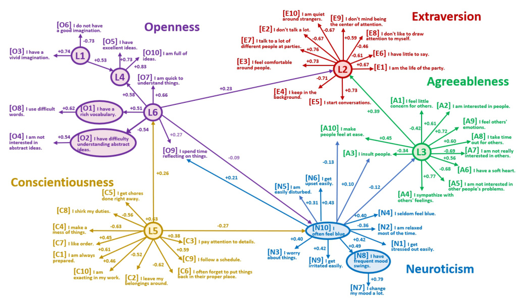
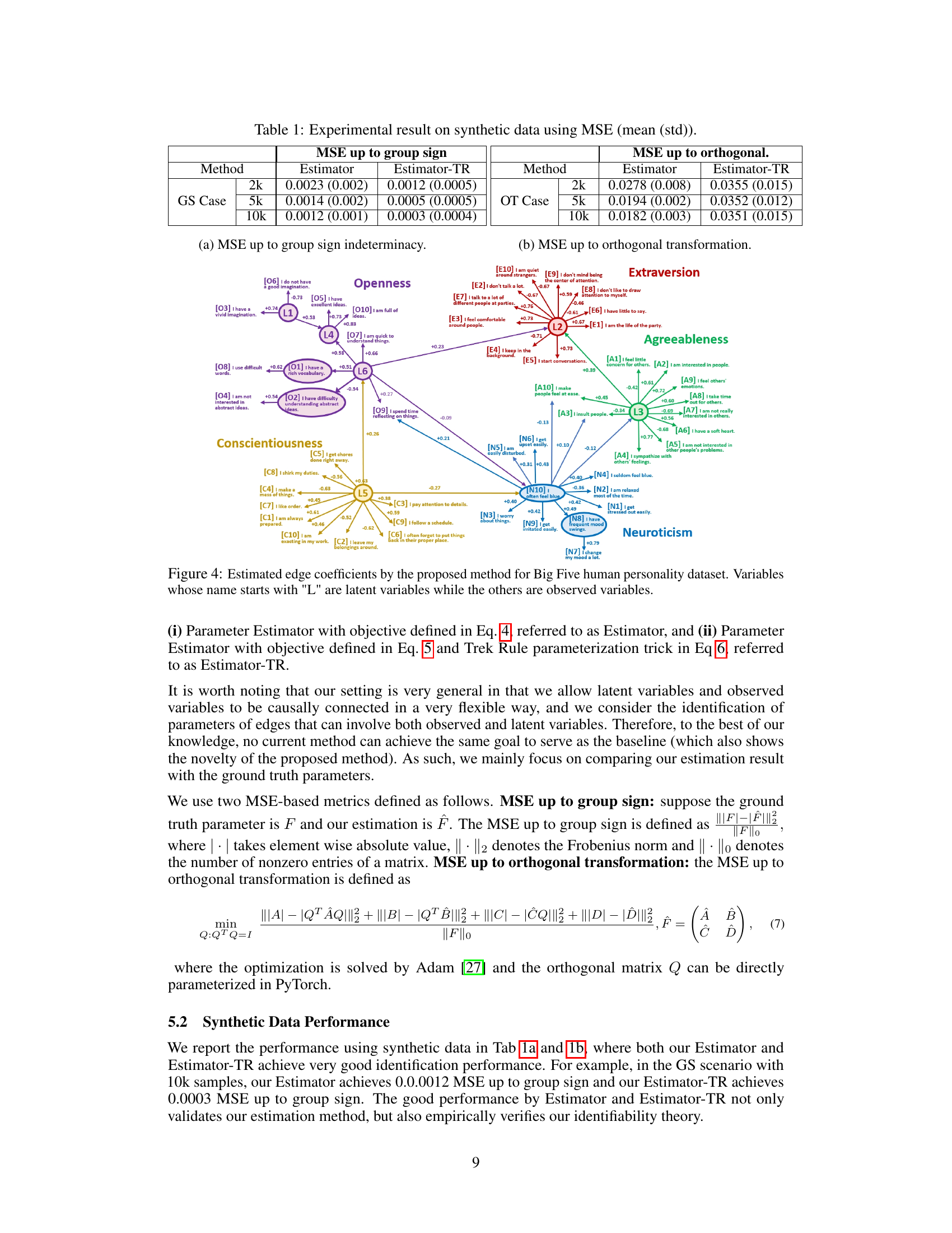
🔼 This figure shows the estimated edge coefficients in a linear causal model representing the Big Five personality traits. The model includes both observed variables (personality traits measured by survey questions) and latent variables (unobserved factors influencing personality). The edge coefficients, which represent the strength of causal relationships between variables, are displayed on the edges connecting the nodes. Positive values suggest a positive relationship, while negative values indicate a negative relationship. The latent variables are denoted by names starting with ‘L’. The figure visually represents the learned causal structure of the personality model and the strength of the direct causal effects between both observed and latent variables.
read the caption
Figure 4: Estimated edge coefficients by the proposed method for Big Five human personality dataset. Variables whose name starts with 'L' are latent variables while the others are observed variables.
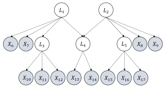
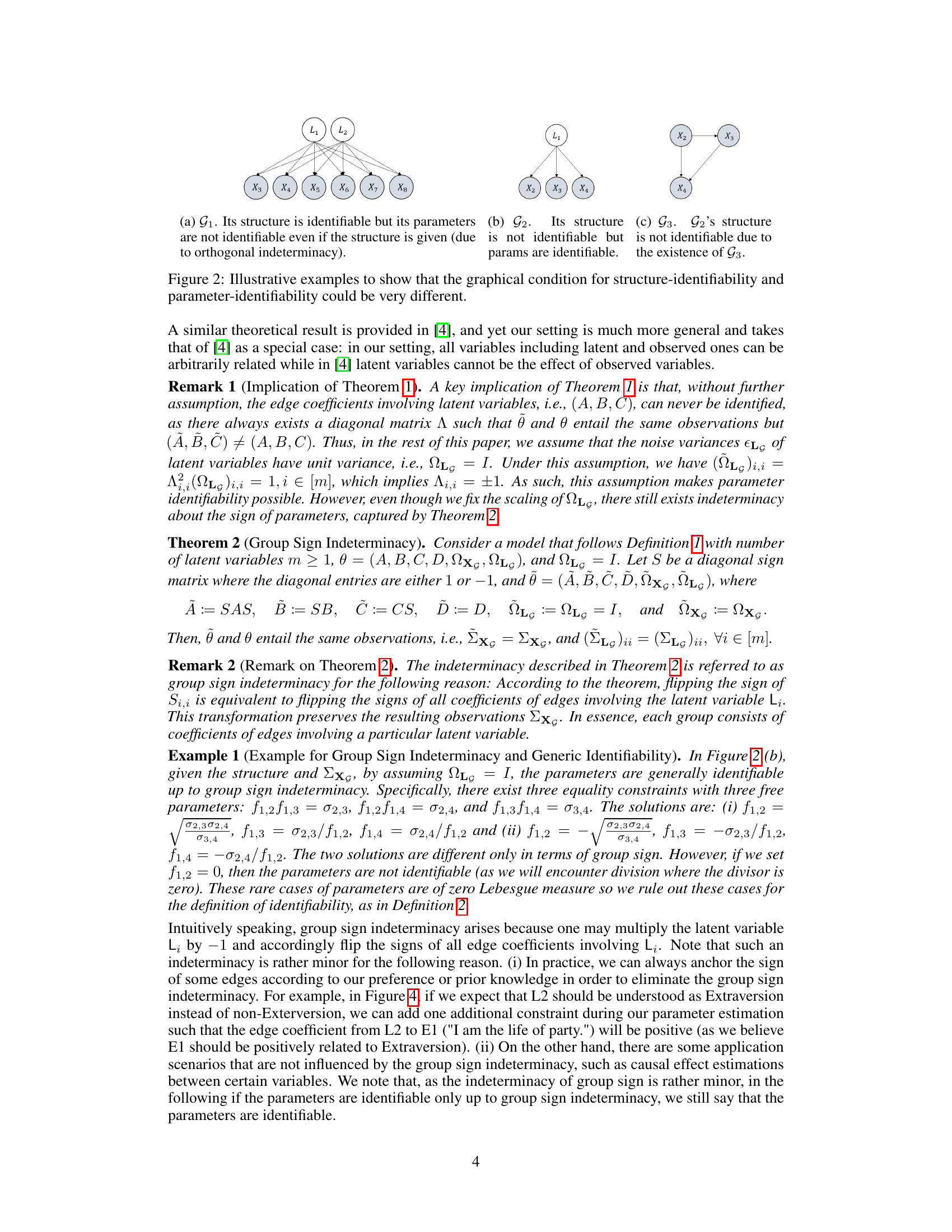
🔼 This figure demonstrates a graph structure where the parameters are not identifiable due to orthogonal transformation indeterminacy. Specifically, the atomic cover {L1, L2} contains more than one latent variable, leading to this indeterminacy affecting the edges connected to L1 and L2. The figure illustrates how the presence of multiple latent variables with identical parents and children causes ambiguity in parameter estimation.
read the caption
Figure 8: An illustrative graph to show orthogonal transformation indeterminacy. An atomic cover of it, {L1, L2}, has more than one latent variable, and thus there exists orthogonal transformation indeterminacy regarding coefficients of edges that involve {L1, L2}.

🔼 This figure compares three graphs to illustrate the advantages of the proposed framework over existing methods. Graph G1 demonstrates a scenario where the parameters are identifiable. Graph G2 shows a scenario where the parameters are not identifiable. Both G1 and G2 are projected into the same ADMG (acyclic directed mixed graph) using the latent projection framework, highlighting a limitation of that approach: it cannot differentiate between identifiable and unidentifiable models when latent variables are involved. The proposed framework overcomes this limitation by considering all variables and edge coefficients, even those involving latent variables.
read the caption
Figure 1: Illustrations of the advantage of our framework. Within our framework, it can be shown that G₁'s parameters can be identified (up to sign) while G2's cannot. In contrast, the latent projection framework cannot even differentiate G₁ from G2 as they share the same ADMG (c) after projection. Furthermore, with ADMG, any edge coefficient that involves a latent variable cannot be considered.

🔼 This figure compares two causal graphs (G1 and G2) and their corresponding ADMG (acyclic directed mixed graph) in the latent projection framework. It highlights that while our proposed framework can identify the parameters of G1 (up to sign), it cannot identify the parameters of G2. The latent projection framework, on the other hand, fails to distinguish between G1 and G2 because they project to the same ADMG. The key difference is that our framework considers edge coefficients involving latent variables, which the latent projection framework does not.
read the caption
Figure 1: Illustrations of the advantage of our framework. Within our framework, it can be shown that G₁'s parameters can be identified (up to sign) while G2's cannot. In contrast, the latent projection framework cannot even differentiate G₁ from G2 as they share the same ADMG (c) after projection. Furthermore, with ADMG, any edge coefficient that involves a latent variable cannot be considered.

🔼 This figure illustrates a graph with latent variables (L1, L2, L3, L4) and observed variables (X1-X18). The key point is that the latent variables L1 and L2 share the same parents (X5, X6) and children (X9-X12). This structure demonstrates orthogonal transformation indeterminacy, meaning that the model parameters (edge coefficients) are not uniquely identifiable. There exists more than one set of parameters that would produce the same observed covariance matrix. This indeterminacy is specifically relevant to the parameters associated with the edges connected to L1 and L2.
read the caption
Figure 8: An illustrative graph to show orthogonal transformation indeterminacy. An atomic cover of it, {L1, L2}, has more than one latent variable, and thus there exists orthogonal transformation indeterminacy regarding coefficients of edges that involve {L1, L2}.

🔼 This figure compares two graphs, G1 and G2, illustrating the difference in identifiability of parameters using different frameworks. G1’s parameters are identifiable (up to a sign ambiguity) within the proposed framework, whereas G2’s parameters are not. The latent projection framework, however, fails to distinguish between G1 and G2 because they produce the same ADMG upon projection, thereby highlighting the limitation of previous frameworks which cannot handle edge coefficients involving latent variables.
read the caption
Figure 1: Illustrations of the advantage of our framework. Within our framework, it can be shown that G₁'s parameters can be identified (up to sign) while G2's cannot. In contrast, the latent projection framework cannot even differentiate G₁ from G2 as they share the same ADMG (c) after projection. Furthermore, with ADMG, any edge coefficient that involves a latent variable cannot be considered.

🔼 This figure compares the proposed framework with the latent projection framework by showing two graphs, G1 and G2. The proposed framework can identify the parameters of G1 (up to sign), while it cannot for G2. The latent projection framework, however, fails to distinguish between G1 and G2 because they produce the same ADMG after projection. This highlights the advantage of the proposed framework in handling latent variables.
read the caption
Figure 1: Illustrations of the advantage of our framework. Within our framework, it can be shown that G₁'s parameters can be identified (up to sign) while G₂'s cannot. In contrast, the latent projection framework cannot even differentiate G₁ from G₂ as they share the same ADMG (c) after projection. Furthermore, with ADMG, any edge coefficient that involves a latent variable cannot be considered.
🔼 This figure compares the proposed framework with existing methods for parameter identifiability in partially observed linear causal models. It shows two graphs, G1 and G2, where G1’s parameters are identifiable while G2’s are not, highlighting the advantage of the proposed framework. The figure also demonstrates that the latent projection framework, which projects the DAG with latent variables onto an ADMG, fails to distinguish between G1 and G2 because it loses crucial information during projection and cannot consider edge coefficients involving latent variables.
read the caption
Figure 1: Illustrations of the advantage of our framework. Within our framework, it can be shown that G₁'s parameters can be identified (up to sign) while G2's cannot. In contrast, the latent projection framework cannot even differentiate G₁ from G2 as they share the same ADMG (c) after projection. Furthermore, with ADMG, any edge coefficient that involves a latent variable cannot be considered.

🔼 This figure illustrates a graph with latent variables L1 and L2 that share the same parents and children. This demonstrates orthogonal transformation indeterminacy, meaning the parameters of the model cannot be uniquely identified due to the existence of multiple equivalent parameterizations.
read the caption
Figure 8: An illustrative graph to show orthogonal transformation indeterminacy. An atomic cover of it, {L1, L2}, has more than one latent variable, and thus there exists orthogonal transformation indeterminacy regarding coefficients of edges that involve {L1, L2}.
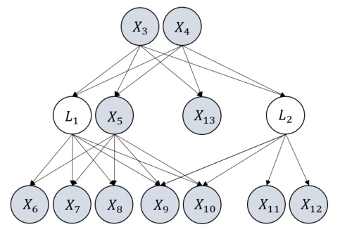
🔼 This figure compares the author’s proposed framework with the latent projection framework using two example graphs, G1 and G2. The figure highlights that the authors’ framework can distinguish between the identifiability of parameters in G1 and G2, while the latent projection framework cannot, as both graphs project to the same ADMG. This demonstrates the advantage of the new framework which allows for the identification of parameters involving latent variables, a limitation of previous methods. The figure showcases how different graph structures can result in different parameter identifiability characteristics.
read the caption
Figure 1: Illustrations of the advantage of our framework. Within our framework, it can be shown that G₁'s parameters can be identified (up to sign) while G₂'s cannot. In contrast, the latent projection framework cannot even differentiate G₁ from G₂ as they share the same ADMG (c) after projection. Furthermore, with ADMG, any edge coefficient that involves a latent variable cannot be considered.

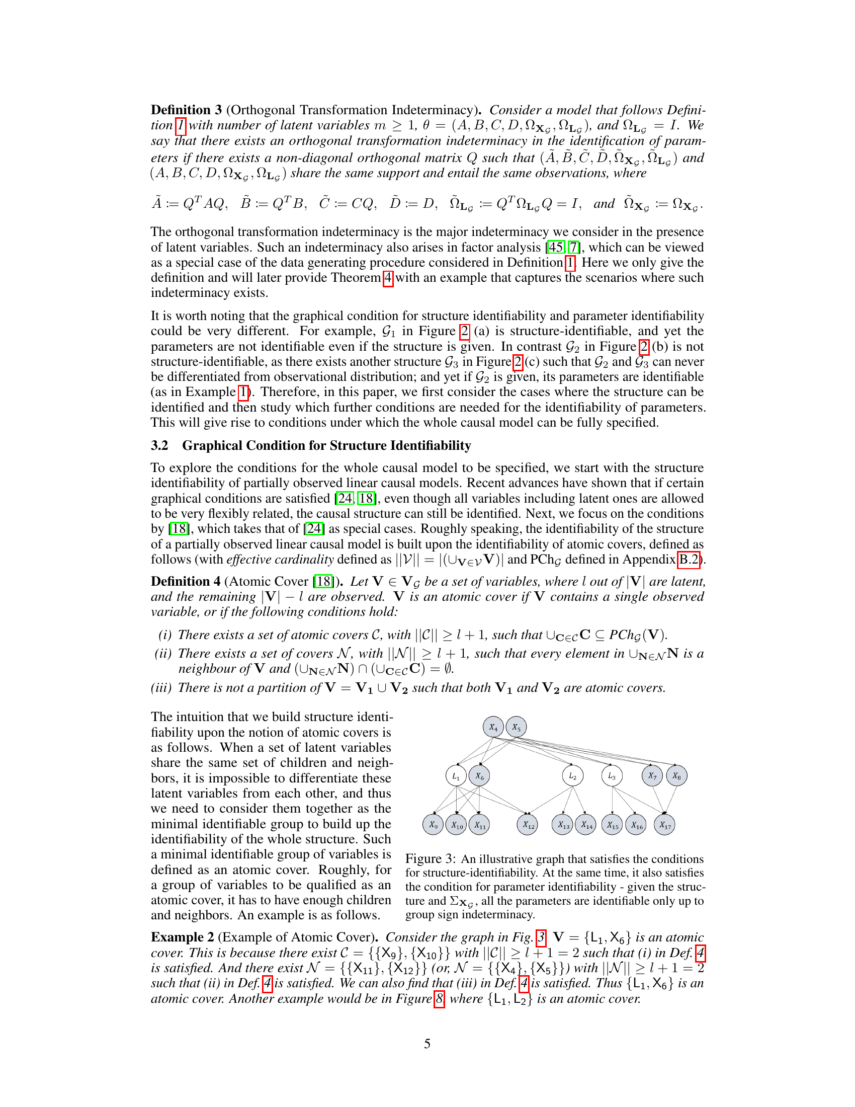
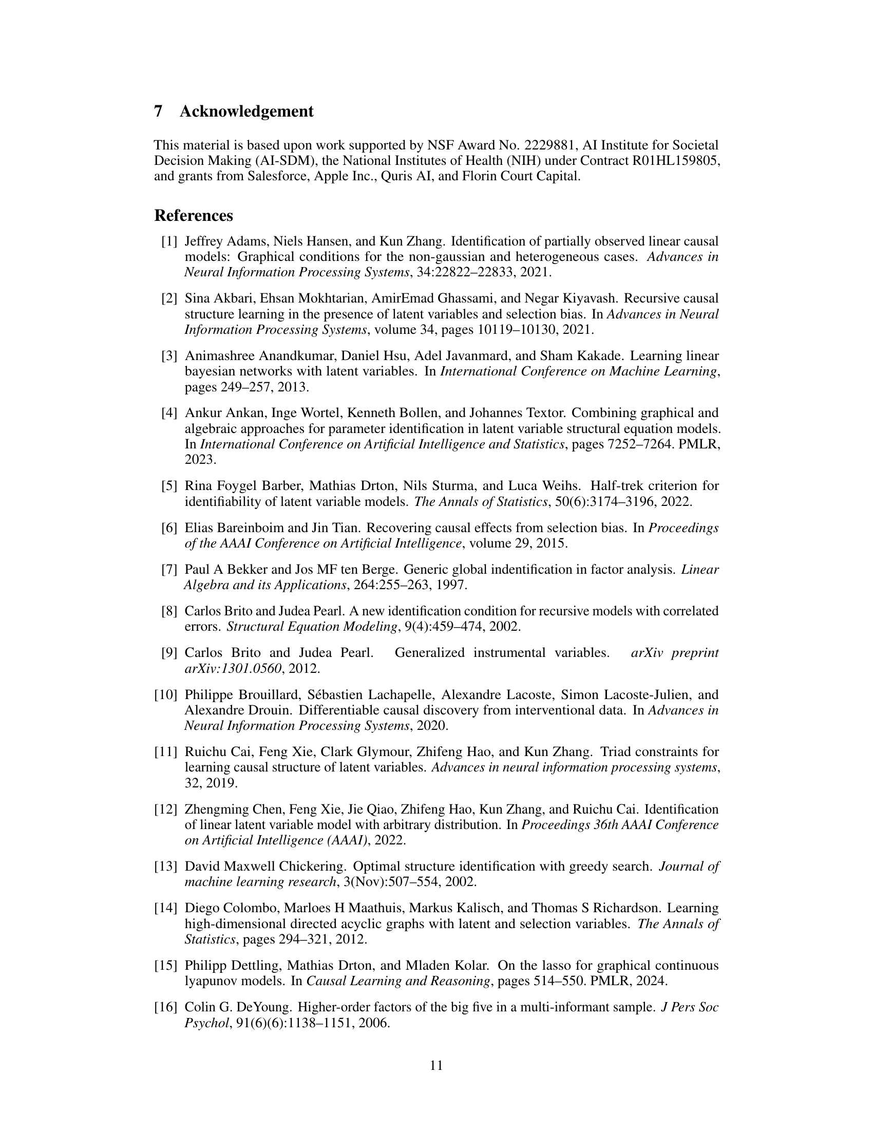
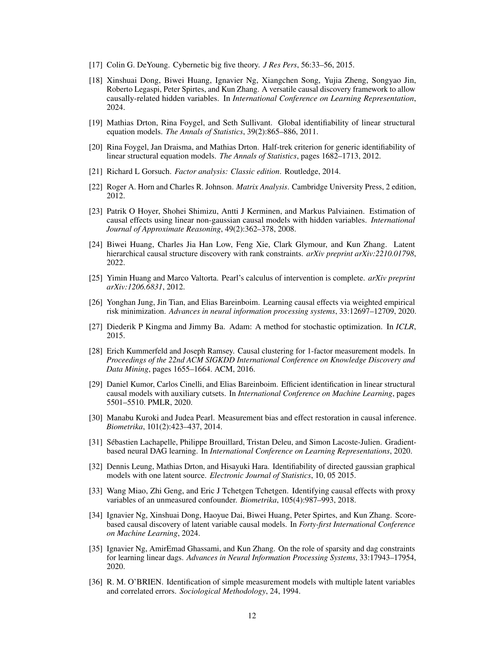
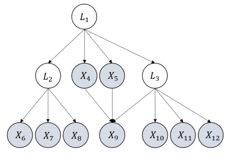
🔼 The figure is an illustrative graph showing a partially observed linear causal model. It demonstrates a model where the structure is identifiable and the parameters are identifiable up to a group sign indeterminacy. The graph includes both observed (X) and latent (L) variables. The conditions for structure identifiability (Condition 1 and 2) and parameter identifiability (Theorem 3) are satisfied by this graph. The figure highlights that all parameters are identifiable up to a group sign.
read the caption
Figure 3: An illustrative graph that satisfies the conditions for structure-identifiability. At the same time, it also satisfies the condition for parameter identifiability - given the structure and Σχ, all the parameters are identifiable only up to group sign indeterminacy.
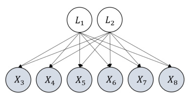
🔼 This figure shows a graph with two latent variables L1 and L2, and six observed variables X3 to X8. The latent variables are parents to all observed variables. The key point is that L1 and L2 share the same children (observed variables), which exemplifies the condition for orthogonal transformation indeterminacy as discussed in the paper. This indeterminacy affects the identifiability of edge coefficients involving these latent variables.
read the caption
Figure 8: An illustrative graph to show orthogonal transformation indeterminacy. An atomic cover of it, {L1, L2}, has more than one latent variable, and thus there exists orthogonal transformation indeterminacy regarding coefficients of edges that involve {L1, L2}.

🔼 This figure illustrates a graph with latent variables L1 and L2 that share the same parents and children. The caption points out that this structure demonstrates orthogonal transformation indeterminacy, meaning the parameters (edge coefficients) cannot be uniquely identified, even if the graph structure and data are known. The indeterminacy specifically affects the coefficients on edges involving L1 and L2.
read the caption
Figure 8: An illustrative graph to show orthogonal transformation indeterminacy. An atomic cover of it, {L1, L2}, has more than one latent variable, and thus there exists orthogonal transformation indeterminacy regarding coefficients of edges that involve {L1, L2}.

🔼 This figure illustrates a graph with latent variables L1 and L2 that share the same parents and children. This structure demonstrates orthogonal transformation indeterminacy, a type of parameter non-identifiability in partially observed linear causal models where multiple parameter sets can produce the same observational data. Specifically, the parameters associated with edges involving L1 and L2 cannot be uniquely determined, only up to an orthogonal transformation.
read the caption
Figure 8: An illustrative graph to show orthogonal transformation indeterminacy. An atomic cover of it, {L1, L2}, has more than one latent variable, and thus there exists orthogonal transformation indeterminacy regarding coefficients of edges that involve {L1, L2}.
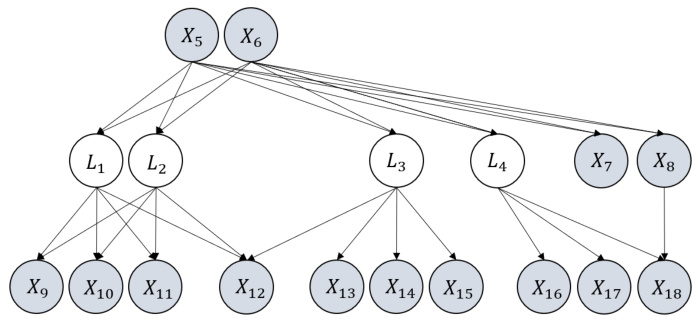
🔼 This figure illustrates a graph with latent variables (L1, L2, L3, L4) and observed variables (X1-X18). The key takeaway is that the atomic cover {L1, L2} has more than one latent variable, which leads to orthogonal transformation indeterminacy. This indeterminacy impacts the identifiability of the parameters (edge coefficients) associated with the edges involving L1 and L2. The figure highlights a scenario where the model’s parameters cannot be uniquely identified, even if the structure is known, due to the presence of multiple latent variables within a single atomic cover.
read the caption
Figure 8: An illustrative graph to show orthogonal transformation indeterminacy. An atomic cover of it, {L1, L2}, has more than one latent variable, and thus there exists orthogonal transformation indeterminacy regarding coefficients of edges that involve {L1, L2}.
More on tables

🔼 This table presents the mean and standard deviation of the Mean Squared Error (MSE) for estimating parameters up to group sign indeterminacy. The experiment uses uniform noise instead of Gaussian noise, violating the normality assumption of the model. The results are shown for different sample sizes (2k, 5k, 10k) and for two different estimators: Estimator and Estimator-TR.
read the caption
Table 2: Performance under violation of normality using uniform noise terms in MSE (mean (std)).

🔼 This table presents the Mean Squared Error (MSE) up to group sign for two different estimators (Estimator and Estimator-TR) under varying degrees of nonlinearity introduced by the leaky ReLU function. The experiment uses the GS case with 10k samples. The results show the MSE under different alpha (α) values, which control the linearity of the leaky ReLU (α=0.8 being close to linear, α=0.6 quite nonlinear, and α=0.3 very nonlinear). It demonstrates the robustness of the estimation methods to deviations from perfect linearity.
read the caption
Table 3: Performance under violation of linearity using leaky relu in MSE (mean (std)).
Full paper#
