↗ arXiv ↗ Hugging Face ↗ Hugging Face ↗ Chat
TL;DR#
Current offline preference optimization methods for LLMs heavily rely on manually designed convex loss functions, limiting exploration of the vast search space. This paper addresses this limitation by proposing LLM-driven objective discovery. This approach uses LLMs to iteratively propose and evaluate new loss functions, leading to the discovery of novel algorithms.
The core contribution is the development and evaluation of a novel algorithm, DiscoPOP, which adaptively blends logistic and exponential losses, demonstrating state-of-the-art performance across multiple tasks, including multi-turn dialogue and summarization. The study also explores the generalizability of LLM-driven objective discovery through a small-scale study for image classification.
Key Takeaways#
Why does it matter?#
This paper is highly important for researchers working on Large Language Model (LLM) alignment and offline preference optimization. It introduces a novel method for automatically discovering new preference optimization algorithms using LLMs, which significantly expands the search space and potentially leads to more efficient and effective alignment techniques. The discovered algorithms are shown to achieve state-of-the-art performance and successfully transfer to held-out tasks, highlighting the effectiveness of this LLM-driven approach.
Visual Insights#

🔼 This figure illustrates the LLM-driven discovery process. The left panel shows a conceptual overview of how the process works: An LLM is prompted to generate new code for offline preference optimization loss functions. These functions are then evaluated, and the results are fed back to the LLM to improve the next proposal. This process iterates until a satisfactory loss function is found. The right panel shows the performance of the discovered objective functions compared to existing baseline methods on the Alpaca Eval benchmark. DiscoPOP shows state-of-the-art performance.
read the caption
Figure 1: Left. Conceptual illustration of LLM-driven discovery of objective functions. We prompt an LLM to output new code-level implementations of offline preference optimization losses E(yw,y1,x)~D [f (βp)] as a function of the policy (πο) and reference model's (ref) likelihoods of the chosen (yw) and rejected (yı) completions. Afterwards, we run an inner loop training procedure and evaluate the resulting model on MT-Bench. The corresponding performance is fed back to the language model, and we query it for the next candidate. Right. Performance of discovered objective functions on Alpaca Eval.

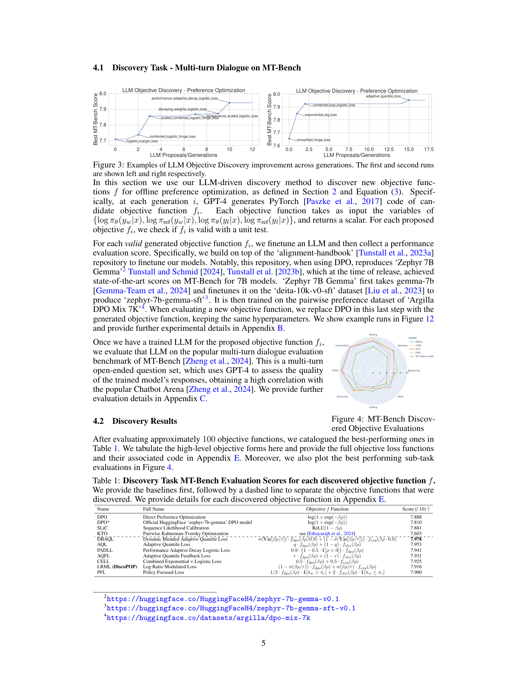
🔼 This table presents the MT-Bench evaluation scores for various offline preference optimization objective functions. It compares the performance of several discovered objective functions against established baseline methods (DPO, SLIC, KTO). The table includes the full name of each objective function, its mathematical representation, and its corresponding MT-Bench score. The discovered objective functions are separated from the baselines by a dashed line for clarity. More detailed information about each objective function can be found in Appendix E.
read the caption
Table 1: Discovery Task MT-Bench Evaluation Scores for each discovered objective function f. We provide the baselines first, followed by a dashed line to separate the objective functions that were discovered. We provide details for each discovered objective function in Appendix E.
In-depth insights#
LLM-driven discovery#
The concept of “LLM-driven discovery” presents a paradigm shift in algorithmic development. By leveraging the capabilities of large language models (LLMs), researchers can automate the process of discovering new algorithms, significantly reducing the reliance on human creativity and intuition. This approach is particularly valuable in complex domains such as preference optimization where the search space for effective loss functions is vast and largely unexplored. The iterative prompting methodology, where the LLM proposes and refines new algorithms based on performance feedback, is a core strength of this method. This allows for the exploration of a broader design space than what is typically possible through manual efforts alone. However, challenges remain. The reliance on the LLM’s internal knowledge base means the discovered algorithms are limited by the LLM’s training data, potentially limiting generalizability and introducing biases. Furthermore, the quality and reliability of the LLM’s suggestions need careful evaluation to ensure that proposed algorithms are indeed novel and effective. Careful validation and testing on diverse datasets are critical for verifying the robustness and generalizability of LLM-discovered algorithms, mitigating potential risks associated with using untested or poorly-understood approaches. In essence, LLM-driven discovery offers a powerful tool, but its effective use requires a thoughtful and rigorous approach that acknowledges and addresses potential limitations.
DiscoPOP algorithm#
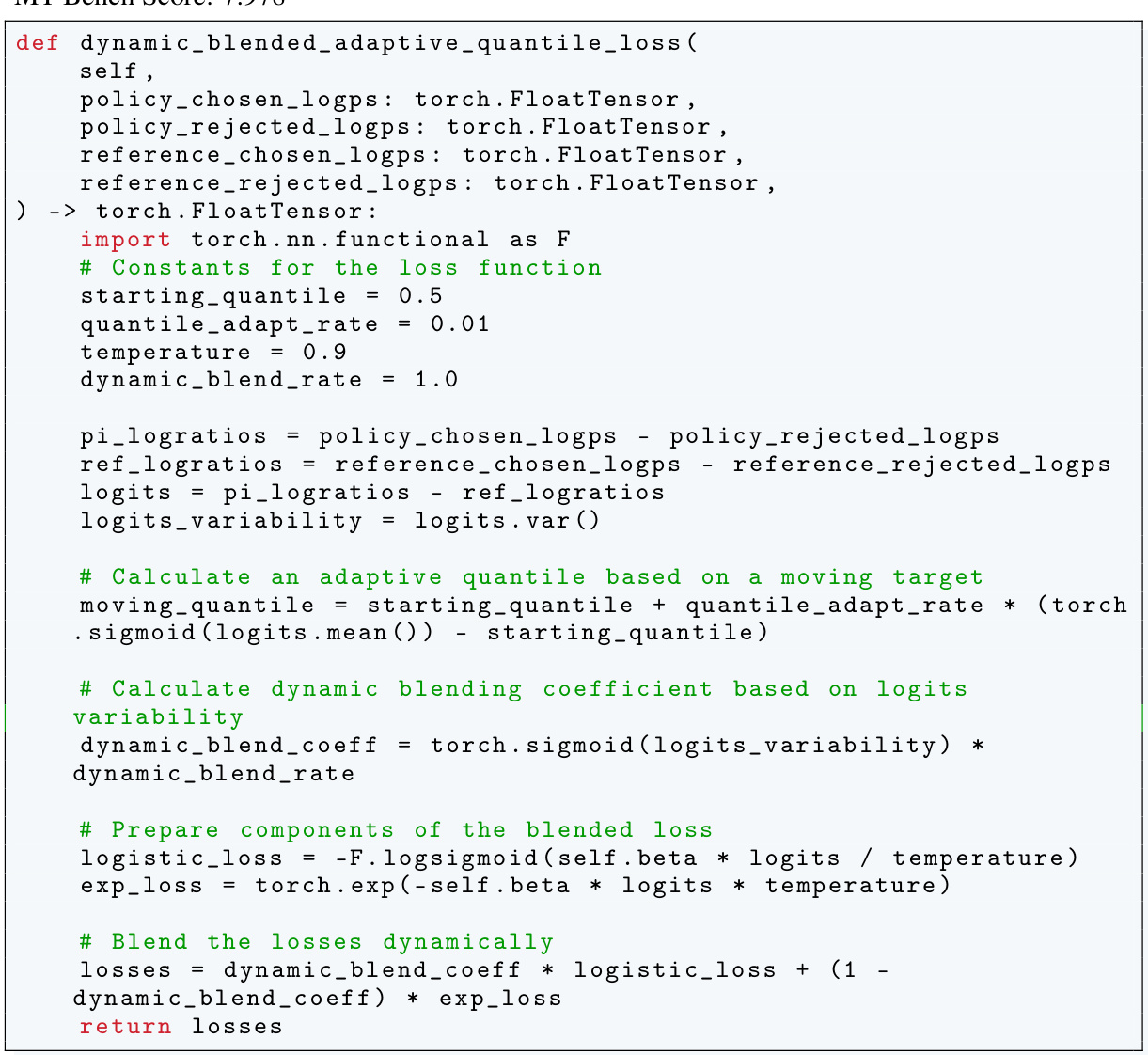
The DiscoPOP algorithm, a novel offline preference optimization algorithm, is a key contribution of this research. It leverages LLM-driven objective discovery, iteratively prompting a language model to propose and refine loss functions based on performance metrics. This approach moves beyond manually designed loss functions, leading to potentially superior performance and exploring a far larger space of optimization strategies. DiscoPOP specifically excels by adaptively blending logistic and exponential losses, dynamically weighting each based on a calculated log-ratio difference. This adaptive strategy proves robust and generalizes well to multiple held-out tasks, showcasing its practical applicability. Non-convexity is a surprising characteristic, suggesting potential advantages over traditional convex methods. While DiscoPOP shows state-of-the-art performance, further investigation is needed to fully understand its properties, including exploring the influence of hyperparameters and addressing limitations like sensitivity to beta values. The algorithm’s innovative use of LLMs represents a significant advancement in the field, highlighting the potential for automated algorithm discovery.
Offline preference opt.#
Offline preference optimization tackles the challenge of aligning large language models (LLMs) with human preferences without the need for extensive online interaction. This is crucial because online reinforcement learning, while effective, can be costly and time-consuming. Instead, offline methods leverage pre-collected preference data, often in the form of pairwise comparisons of LLM outputs. The core challenge lies in designing effective loss functions that translate these preferences into model updates. Traditional approaches rely on handcrafted convex loss functions, but these are limited by human ingenuity and may not fully explore the vast space of possible functions. Recent research focuses on automated methods for discovering novel loss functions, potentially using techniques like evolutionary algorithms or large language models (LLMs) themselves to guide the search for optimal loss functions. This automated approach holds the promise of significantly advancing offline preference optimization, leading to higher-quality and more aligned LLMs.
Held-out evaluations#
A held-out evaluation section in a research paper is crucial for establishing the generalizability and robustness of a model or method. It assesses performance on unseen data, providing a more realistic picture of real-world applicability beyond the training set. A strong held-out evaluation should include multiple diverse datasets to avoid overfitting to specific characteristics of a single benchmark. The choice of held-out datasets should be carefully justified, reflecting the target application domain and potential biases. Quantitative metrics, such as accuracy or precision, alongside qualitative analyses are necessary for a complete assessment. The comparison to strong baseline models is also essential to showcase the genuine improvement offered by the novel approach. Reporting statistical significance measures, including confidence intervals, further enhances the reliability of findings. Finally, a discussion of potential limitations that might have affected the held-out results is important for providing context and directing future research.
DiscoPOP analysis#
A DiscoPOP analysis would delve into the algorithm’s mechanics, dissecting its adaptive blending of logistic and exponential loss functions. Key aspects to explore include the non-convex nature of the loss landscape and its implications for optimization. The analysis should investigate how the weighting mechanism, determined by a sigmoid function of the log-ratio difference, dynamically balances the two loss components, potentially explaining its superior performance over existing methods. A thorough examination of the algorithm’s sensitivity to hyperparameters, particularly the temperature parameter and beta, would be crucial, as would be an investigation into its robustness and generalization capabilities across different tasks and datasets. Empirical results from diverse evaluation tasks, such as single-turn and multi-turn dialogue, summarization, and sentiment generation, should be analyzed to assess DiscoPOP’s overall effectiveness and its strengths and weaknesses compared to other approaches. Furthermore, the analysis should consider potential limitations of DiscoPOP, such as computational cost or convergence challenges, and propose avenues for future improvements, including strategies to enhance its stability and address any observed limitations.
More visual insights#
More on figures

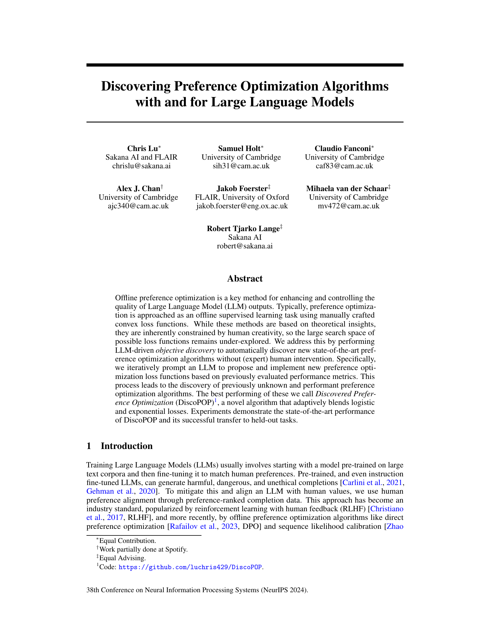
🔼 This figure shows the results of using LLMs to discover new objective functions for image classification on the CIFAR-10 dataset. The left panel shows how the LLM iteratively proposes new loss functions, evaluating their performance and refining its proposals based on the results. This demonstrates the LLM’s ability to explore and combine different concepts to improve performance. The right panel shows that the three best-performing discovered objective functions generalize well to different network architectures (ResNet18, SimpleDLA, EfficientNetB0) and longer training times (100 epochs).
read the caption
Figure 2: LLM-driven objective discovery for CIFAR-10 classification. Left. Performance across LLM-discovery trials. The proposals alternate between exploring new objective concepts, tuning the components, and combining previous insights. Right. The best three discovered objectives transfer to different network architectures and longer training runs (100 epochs).

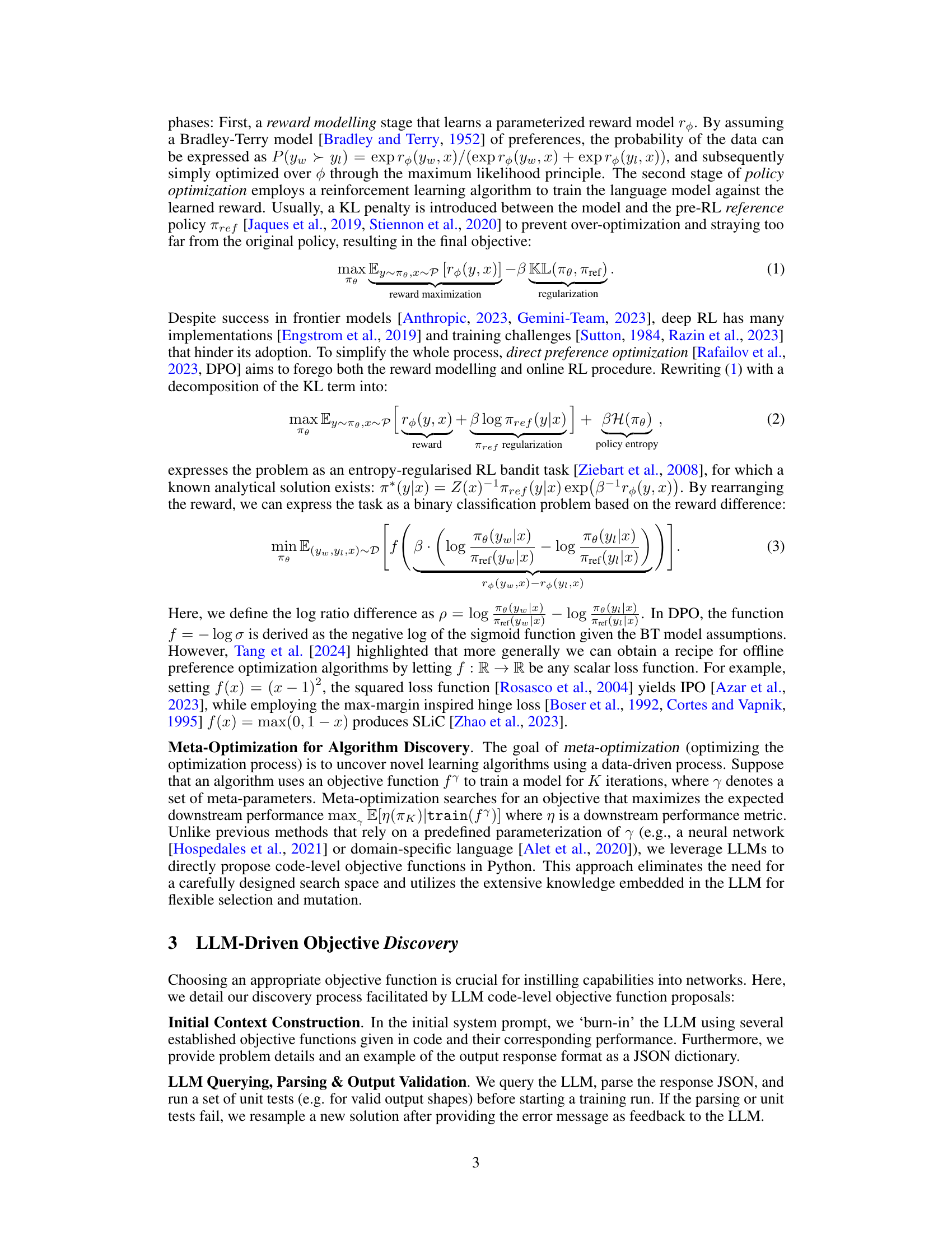
🔼 This figure shows two examples of how the LLM-driven objective discovery method improves the performance of the objective functions across multiple generations. The left panel shows the first run, which starts with several baseline objective functions and then iteratively proposes and evaluates new objective functions based on feedback from the performance of the models trained with those functions. The right panel shows a second run which demonstrates a similar improvement in performance as the number of generations increase. The x-axis represents the number of generations in the objective discovery process, and the y-axis represents the best MT-Bench score achieved in each generation.
read the caption
Figure 3: Examples of LLM Objective Discovery improvement across generations. The first and second runs are shown left and right respectively.

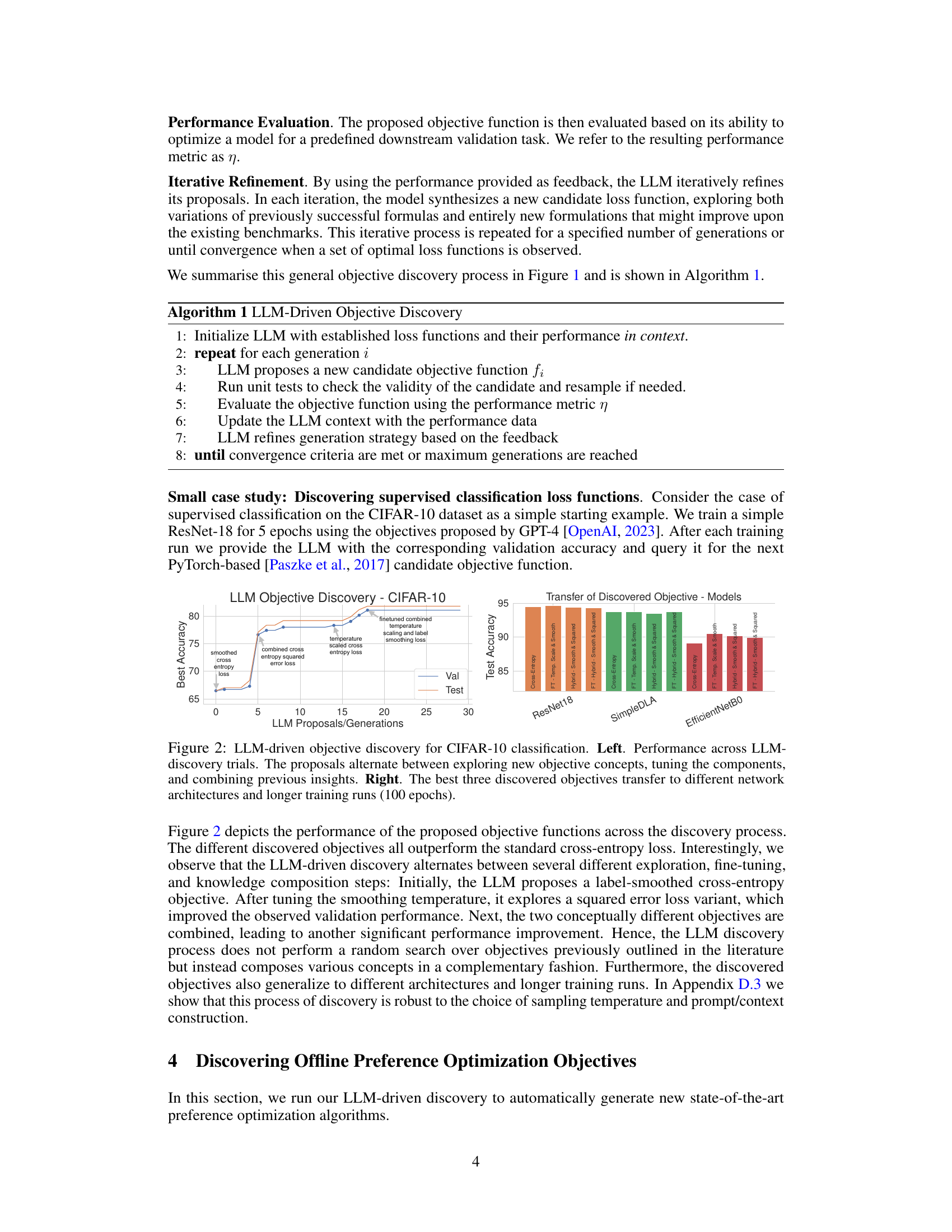
🔼 This radar chart visualizes the performance of different models trained with various objective functions on the MT-Bench benchmark. Each axis represents a sub-task within MT-Bench (Humanities, STEM, Extraction, Writing, Coding, Roleplay, Reasoning, Math). The length of each line extending from the center to the outer edge indicates the model’s performance on that particular sub-task, with higher values signifying better performance. The different colored lines represent different models: PADLL, LRML (DiscoPOP), SLIC, DPO, and the SFT base model. The chart allows for a quick comparison of the relative strengths and weaknesses of each model across the various sub-tasks of the MT-Bench evaluation.
read the caption
Figure 4: MT-Bench Discovered Objective Evaluations
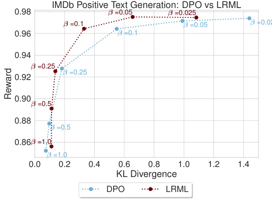
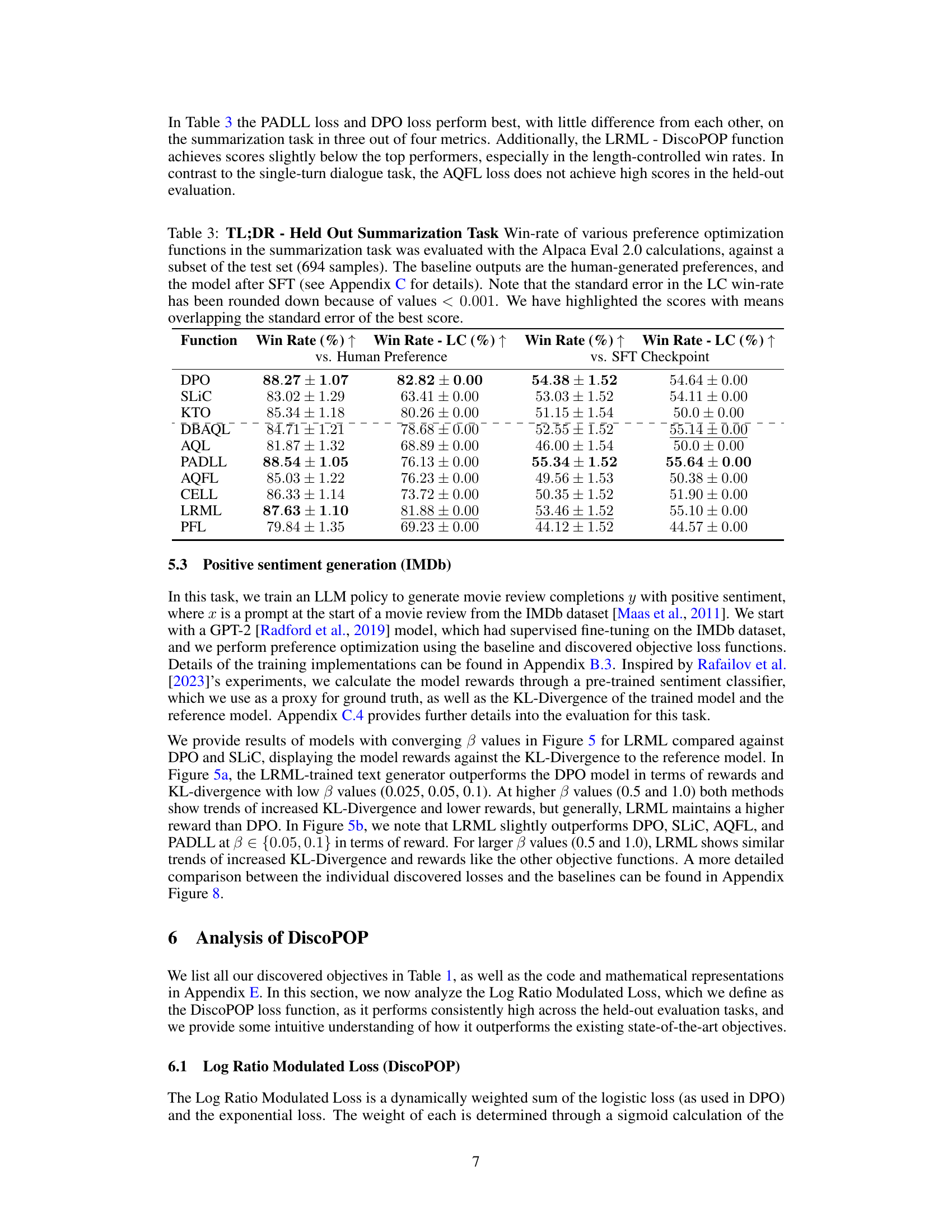
🔼 This figure shows the trade-off between expected reward and KL divergence from a reference model for different beta values (β) across multiple generations. The plot shows the performance of three different objective functions: LRML (the discovered objective function), DPO, and SLiC. The top-left corner represents the ideal scenario—high reward with minimal divergence from the reference model, indicating effective alignment. The plot illustrates how each objective function balances reward and model divergence at different β values. The plot is useful for comparing the performance of the new objective function (LRML) with existing baselines (DPO and SLiC).
read the caption
Figure 5: Frontiers of expected reward vs KL divergence for converging models for the LRML against DPO and SLiC objective function. The rewards and KL-divergence values are averaged over 10 generations with different seeds. The sweep is done over β∈ {0.025, 0.05, 0.1, 0.25, 0.5, 1.0}. The optimal point is the top left corner, where the perfect reward is achieved with minimal divergence from the reference model.

🔼 This figure shows the Pareto frontier of expected reward vs. KL divergence for different optimization objective functions. The x-axis represents the KL divergence between the trained model and the reference model, while the y-axis represents the expected reward. Each point represents the average performance over 10 generations with different random seeds. The different colors represent different objective functions. The optimal performance would be in the top-left corner, where the reward is high and the KL divergence is low. The figure shows that LRML outperforms DPO and SLIC objective functions on this metric.
read the caption
Figure 5: Frontiers of expected reward vs KL divergence for converging models for the LRML against DPO and SLiC objective function. The rewards and KL-divergence values are averaged over 10 generations with different seeds. The sweep is done over β∈ {0.025, 0.05, 0.1, 0.25, 0.5, 1.0}. The optimal point is the top left corner, where the perfect reward is achieved with minimal divergence from the reference model.

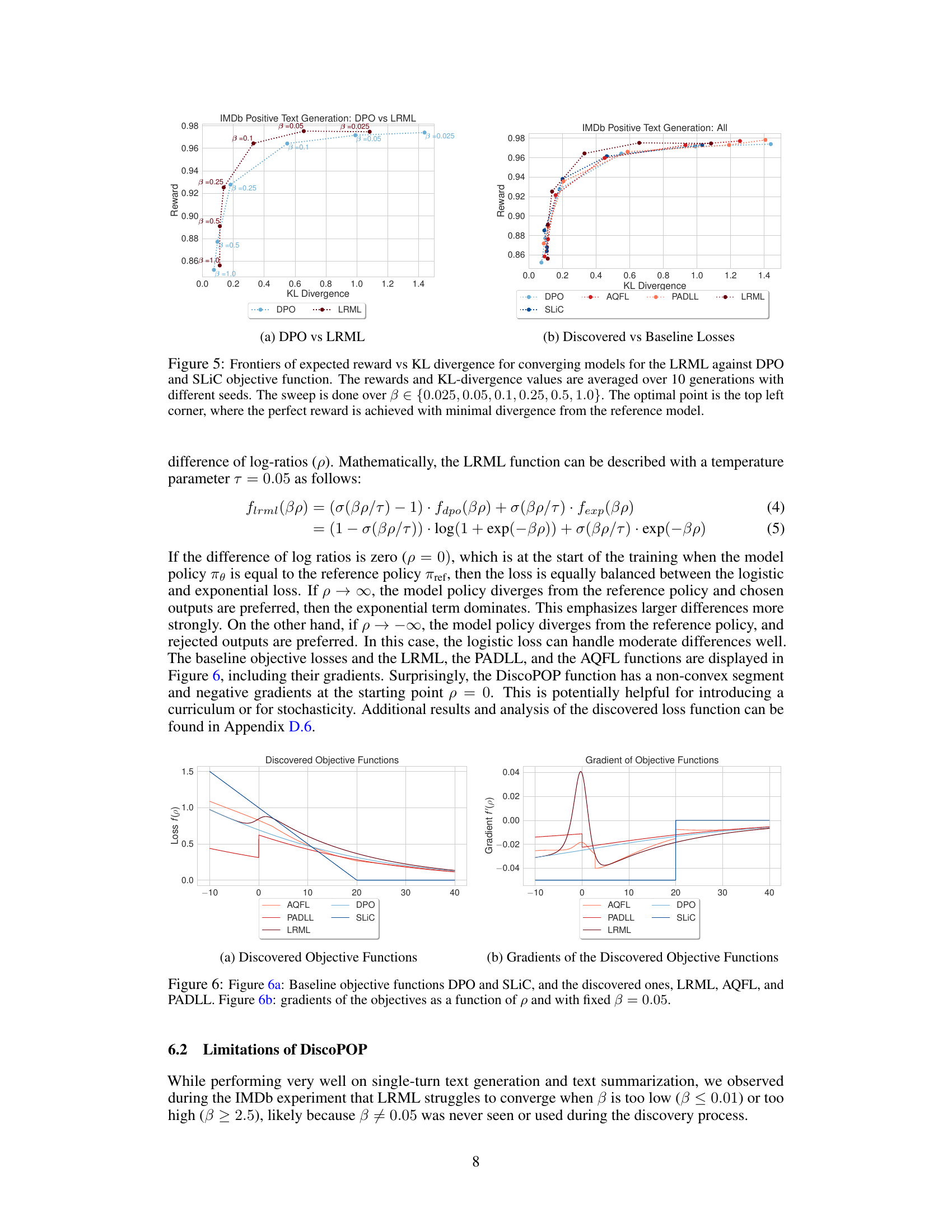
🔼 This figure shows the plots of baseline objective functions (DPO and SLiC) and discovered objective functions (LRML, AQFL, and PADLL) and their gradients. The x-axis represents the log ratio difference (p), and the y-axis represents the loss function value or its gradient. The plots illustrate the shape and behavior of these functions, highlighting differences between baseline and discovered algorithms, and showing the non-convexity of DiscoPOP.
read the caption
Figure 6: Figure 6a: Baseline objective functions DPO and SLiC, and the discovered ones, LRML, AQFL, and PADLL. Figure 6b: gradients of the objectives as a function of p and with fixed β = 0.05.
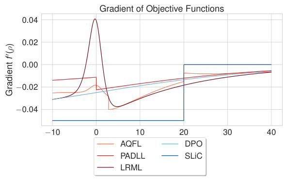
🔼 This figure compares the baseline objective functions (DPO and SLIC) with the discovered ones (LRML, AQFL, and PADLL). Subfigure (a) shows the objective functions themselves plotted against the log ratio difference (p). Subfigure (b) shows the gradients of those same functions, also plotted against p, using a fixed beta value of 0.05. This allows for a visual comparison of the shape and behavior of each function and its gradient, providing insight into their respective properties and how they might affect the optimization process.
read the caption
Figure 6: Figure 6a: Baseline objective functions DPO and SLiC, and the discovered ones, LRML, AQFL, and PADLL. Figure 6b: gradients of the objectives as a function of p and with fixed β = 0.05.
🔼 The figure illustrates the LLM-driven discovery process. The left panel shows a conceptual overview of how an LLM is prompted to propose new loss functions for offline preference optimization. These functions are then evaluated, and the results are fed back to the LLM to iteratively improve the proposed functions. The right panel shows a comparison of the performance of the discovered objective functions against existing baseline methods on the Alpaca Eval benchmark.
read the caption
Figure 1: Left. Conceptual illustration of LLM-driven discovery of objective functions. We prompt an LLM to output new code-level implementations of offline preference optimization losses E(yw,y1,x)~D [f (βp)] as a function of the policy (πο) and reference model's (ref) likelihoods of the chosen (yw) and rejected (yı) completions. Afterwards, we run an inner loop training procedure and evaluate the resulting model on MT-Bench. The corresponding performance is fed back to the language model, and we query it for the next candidate. Right. Performance of discovered objective functions on Alpaca Eval.

🔼 This figure illustrates the LLM-driven objective discovery process. The left panel shows a conceptual diagram of how the LLM proposes new objective functions, trains a model with them, evaluates the performance, and uses the results to inform the next proposal. The right panel presents a bar chart comparing the performance of the discovered objective functions against existing baselines on the Alpaca Eval benchmark.
read the caption
Figure 1: Left. Conceptual illustration of LLM-driven discovery of objective functions. We prompt an LLM to output new code-level implementations of offline preference optimization losses E(yw,y1,x)~D [f (βp)] as a function of the policy (πο) and reference model's (ref) likelihoods of the chosen (yw) and rejected (yı) completions. Afterwards, we run an inner loop training procedure and evaluate the resulting model on MT-Bench. The corresponding performance is fed back to the language model, and we query it for the next candidate. Right. Performance of discovered objective functions on Alpaca Eval.

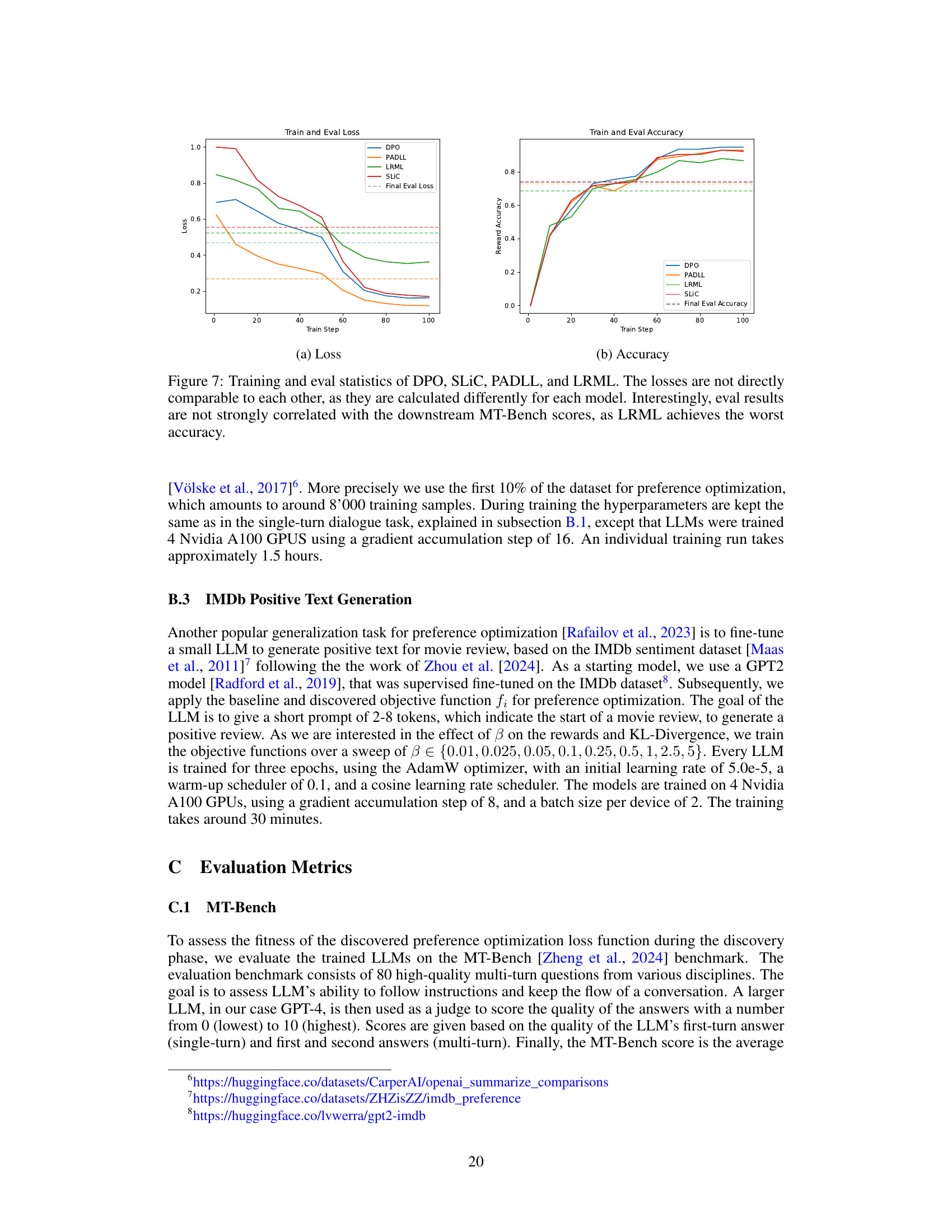
🔼 The figure shows training and evaluation loss and accuracy curves for four different offline preference optimization algorithms (DPO, SLIC, PADLL, LRML) on a specific task. It highlights that while the training losses and accuracies vary considerably among the algorithms, there is not a strong correlation between the evaluation metrics and the final MT-Bench scores, which are used as the primary performance measure.
read the caption
Figure 7: Training and eval statistics of DPO, SLIC, PADLL, and LRML. The losses are not directly comparable to each other, as they are calculated differently for each model. Interestingly, eval results are not strongly correlated with the downstream MT-Bench scores, as LRML achieves the worst accuracy.
🔼 This figure illustrates the LLM-driven objective function discovery process. The left panel shows a flowchart of the process, starting with prompting an LLM to generate a new loss function, followed by an inner loop for training and evaluation, feeding the results back to the LLM for refinement. The right panel presents a bar chart comparing the performance of discovered objective functions against established baselines on the Alpaca Eval benchmark.
read the caption
Figure 1: Left. Conceptual illustration of LLM-driven discovery of objective functions. We prompt an LLM to output new code-level implementations of offline preference optimization losses E(yw,y1,x)~D [f (βp)] as a function of the policy (πο) and reference model's (ref) likelihoods of the chosen (yw) and rejected (yı) completions. Afterwards, we run an inner loop training procedure and evaluate the resulting model on MT-Bench. The corresponding performance is fed back to the language model, and we query it for the next candidate. Right. Performance of discovered objective functions on Alpaca Eval.

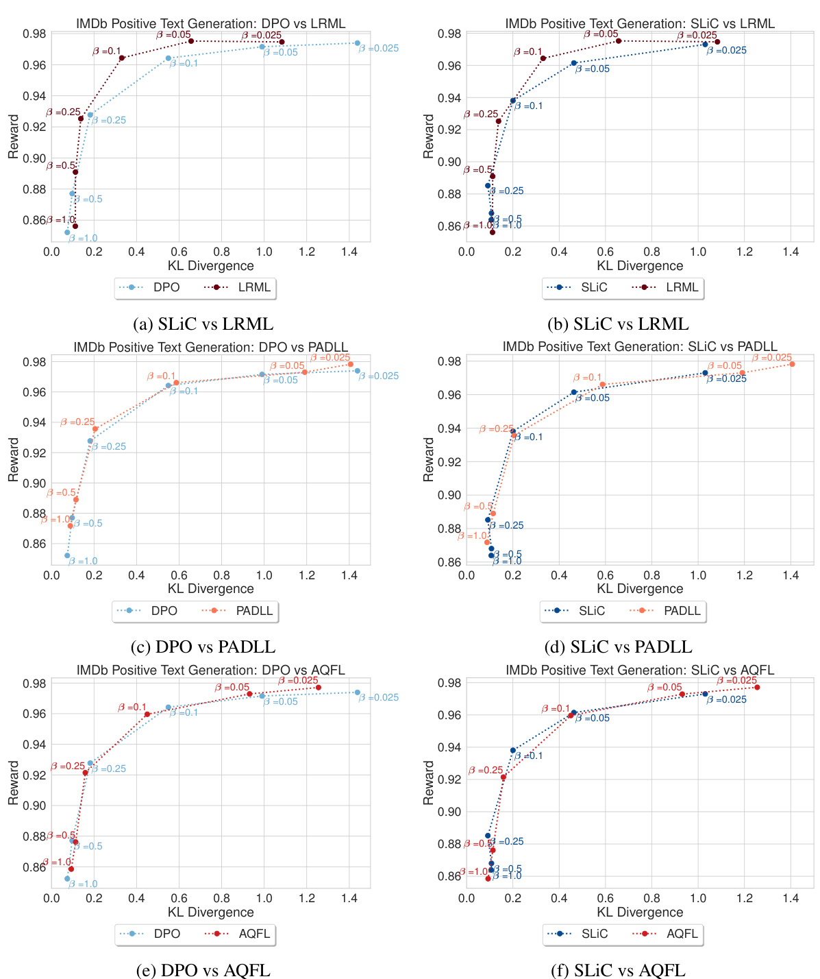
🔼 This figure shows the trade-off between reward and KL divergence for different beta values (β) across various objective functions. The objective functions include baselines (DPO, SLIC) and several novel ones discovered by the LLM. The top-left corner represents the ideal scenario: high reward with minimal KL divergence (meaning the model’s policy is close to the reference policy). Each subplot represents a different beta value, showing how the trade-off changes based on the chosen optimization objective. This helps in understanding the relative strengths of each objective function in balancing reward maximization and maintaining alignment with the pre-trained reference model.
read the caption
Figure 8: Frontiers of expected reward vs KL divergence after convergence for the baseline functions and all the discovered ones. The rewards and KL divergence values are averaged over 10 generations with different seeds. The sweep is done over β∈ {0.025, 0.05, 0.1, 0.25, 0.5, 1, }. The optimal point is the top left corner, where perfect reward is achieved with minimal divergence from the reference model, to avoid reward hacking.

🔼 This figure illustrates the LLM-driven discovery process. The left panel shows a conceptual overview of the process: an LLM is prompted to generate code for a new offline preference optimization loss function, this loss function is then evaluated via model training on MT-Bench, and the performance is fed back to the LLM to inform the next iteration. The right panel shows a bar chart comparing the performance of discovered loss functions against existing baselines on Alpaca Eval.
read the caption
Figure 1: Left. Conceptual illustration of LLM-driven discovery of objective functions. We prompt an LLM to output new code-level implementations of offline preference optimization losses E(yw,y1,x)~D [f (βp)] as a function of the policy (πο) and reference model's (ref) likelihoods of the chosen (yw) and rejected (yı) completions. Afterwards, we run an inner loop training procedure and evaluate the resulting model on MT-Bench. The corresponding performance is fed back to the language model, and we query it for the next candidate. Right. Performance of discovered objective functions on Alpaca Eval.

🔼 This figure illustrates the LLM-driven discovery process. The left panel shows a conceptual diagram of how the process works: an LLM is prompted to generate new loss functions for offline preference optimization. These functions are then evaluated, and their performance is fed back to the LLM to inform the generation of the next candidate. The right panel shows the performance of the discovered loss functions on AlpacaEval, a benchmark for evaluating language models.
read the caption
Figure 1: Left. Conceptual illustration of LLM-driven discovery of objective functions. We prompt an LLM to output new code-level implementations of offline preference optimization losses E(yw,y1,x)~D [f (βp)] as a function of the policy (πο) and reference model's (ref) likelihoods of the chosen (yw) and rejected (yı) completions. Afterwards, we run an inner loop training procedure and evaluate the resulting model on MT-Bench. The corresponding performance is fed back to the language model, and we query it for the next candidate. Right. Performance of discovered objective functions on Alpaca Eval.
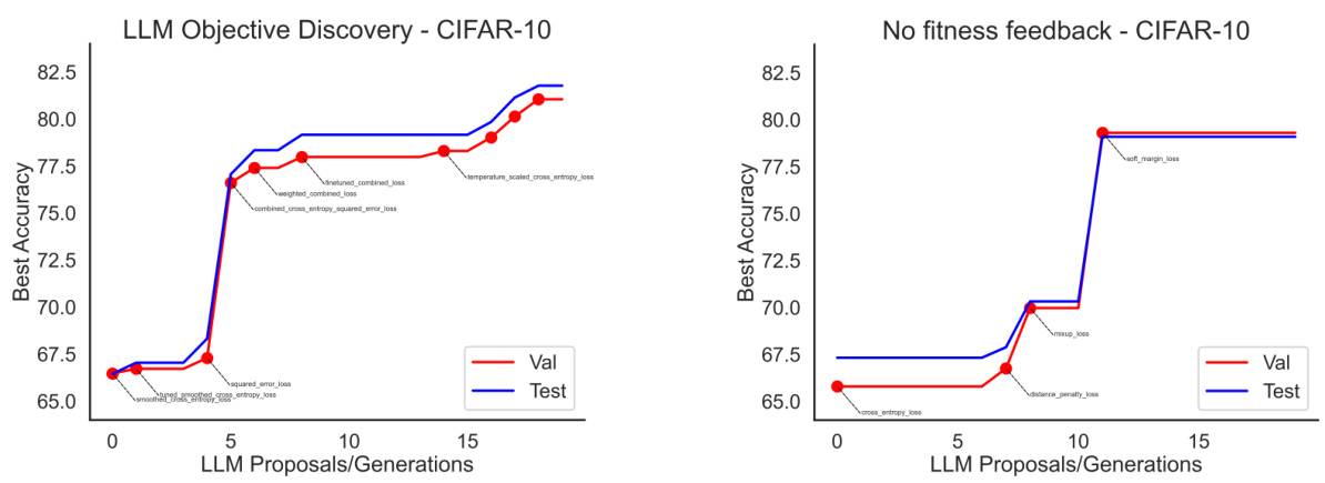
🔼 This figure shows the results of using LLMs to discover new objective functions for CIFAR-10 image classification. The left panel shows the performance of the discovered objectives across multiple generations, highlighting the iterative refinement process where the LLM proposes new objectives, evaluates them, and incorporates the feedback into subsequent proposals. The right panel demonstrates the generalizability of the three best-performing discovered objectives by evaluating their performance on different network architectures (ResNet18, SimpleDLA, and EfficientNetB0) and with longer training runs (100 epochs).
read the caption
Figure 2: LLM-driven objective discovery for CIFAR-10 classification. Left. Performance across LLM-discovery trials. The proposals alternate between exploring new objective concepts, tuning the components, and combining previous insights. Right. The best three discovered objectives transfer to different network architectures and longer training runs (100 epochs).

🔼 The figure illustrates the LLM-driven discovery process. The left panel shows a conceptual overview of how the LLM is prompted to generate new objective functions for offline preference optimization, which are then evaluated in an inner loop, and the results fed back to the LLM to iteratively refine the process. The right panel shows the performance of the discovered objective functions compared to existing baselines on the Alpaca Eval benchmark.
read the caption
Figure 1: Left. Conceptual illustration of LLM-driven discovery of objective functions. We prompt an LLM to output new code-level implementations of offline preference optimization losses E(yw,y1,x)~D [f (βp)] as a function of the policy (πο) and reference model's (ref) likelihoods of the chosen (yw) and rejected (yı) completions. Afterwards, we run an inner loop training procedure and evaluate the resulting model on MT-Bench. The corresponding performance is fed back to the language model, and we query it for the next candidate. Right. Performance of discovered objective functions on Alpaca Eval.
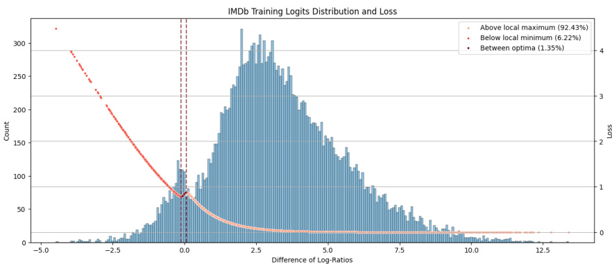
🔼 This figure shows the distribution of β-scaled differences of log-ratios and their corresponding DiscoPOP loss values for the IMDb positive review generation task. The x-axis represents the difference of log-ratios, and the left y-axis shows the count of samples falling into each bin. The right y-axis represents the DiscoPOP loss value. The distribution shows a concentration of samples near zero difference, along with a smaller number of samples at either extreme end. The figure also highlights three key regions: Above local maximum, Between optima, and Below local minimum. The percentage of samples within these regions are stated in the legend. The presence of local optima suggests that the loss function is non-convex and may lead to finding different solutions depending on the initialization.
read the caption
Figure 14: Distribution of β-scaled difference of log-ratios (left y-axis) and corresponding DiscoPOP loss value (right y-axis) of the training samples on the IMDb positive review generation task. The DiscoPOP function has a local minimum at fLRML(-2.3714) = 0.785929 and a local maximum at fLRML(1.44012) = 0.87829. The number of samples within the two local optima corresponds to 1.35% of the training set.
🔼 This figure illustrates the LLM-driven discovery process. The left panel shows a conceptual overview of how the process works: an LLM is prompted to generate code for new loss functions, these functions are then evaluated, and the results are fed back to the LLM to inform the next iteration. The right panel shows a comparison of the performance of various objective functions discovered using this method against established baseline methods on the Alpaca Eval benchmark.
read the caption
Figure 1: Left. Conceptual illustration of LLM-driven discovery of objective functions. We prompt an LLM to output new code-level implementations of offline preference optimization losses E(yw,y1,x)~D [f (βp)] as a function of the policy (πο) and reference model's (ref) likelihoods of the chosen (yw) and rejected (yı) completions. Afterwards, we run an inner loop training procedure and evaluate the resulting model on MT-Bench. The corresponding performance is fed back to the language model, and we query it for the next candidate. Right. Performance of discovered objective functions on Alpaca Eval.
🔼 This figure illustrates the LLM-driven discovery process. The left panel shows a conceptual diagram of how an LLM is prompted to generate new objective functions for offline preference optimization, which are then evaluated, and the results fed back to the LLM for iterative refinement. The right panel shows the performance comparison of different discovered objective functions on Alpaca Eval, demonstrating the discovery of new, high-performing algorithms.
read the caption
Figure 1: Left. Conceptual illustration of LLM-driven discovery of objective functions. We prompt an LLM to output new code-level implementations of offline preference optimization losses E(yw,y1,x)~D [f (βp)] as a function of the policy (πο) and reference model's (ref) likelihoods of the chosen (yw) and rejected (yı) completions. Afterwards, we run an inner loop training procedure and evaluate the resulting model on MT-Bench. The corresponding performance is fed back to the language model, and we query it for the next candidate. Right. Performance of discovered objective functions on Alpaca Eval.

🔼 The figure illustrates the LLM-driven discovery process of objective functions for offline preference optimization. The left panel shows a conceptual diagram of the process: an LLM is prompted to suggest new loss functions, the performance of which is evaluated, and then the feedback is given back to the LLM, creating an iterative process. The right panel shows a bar chart comparing the performance of several objective functions discovered by the LLM against existing baselines on the Alpaca Eval benchmark.
read the caption
Figure 1: Left. Conceptual illustration of LLM-driven discovery of objective functions. We prompt an LLM to output new code-level implementations of offline preference optimization losses E(yw,y1,x)~D [f (βp)] as a function of the policy (πο) and reference model's (ref) likelihoods of the chosen (yw) and rejected (yı) completions. Afterwards, we run an inner loop training procedure and evaluate the resulting model on MT-Bench. The corresponding performance is fed back to the language model, and we query it for the next candidate. Right. Performance of discovered objective functions on Alpaca Eval.
More on tables

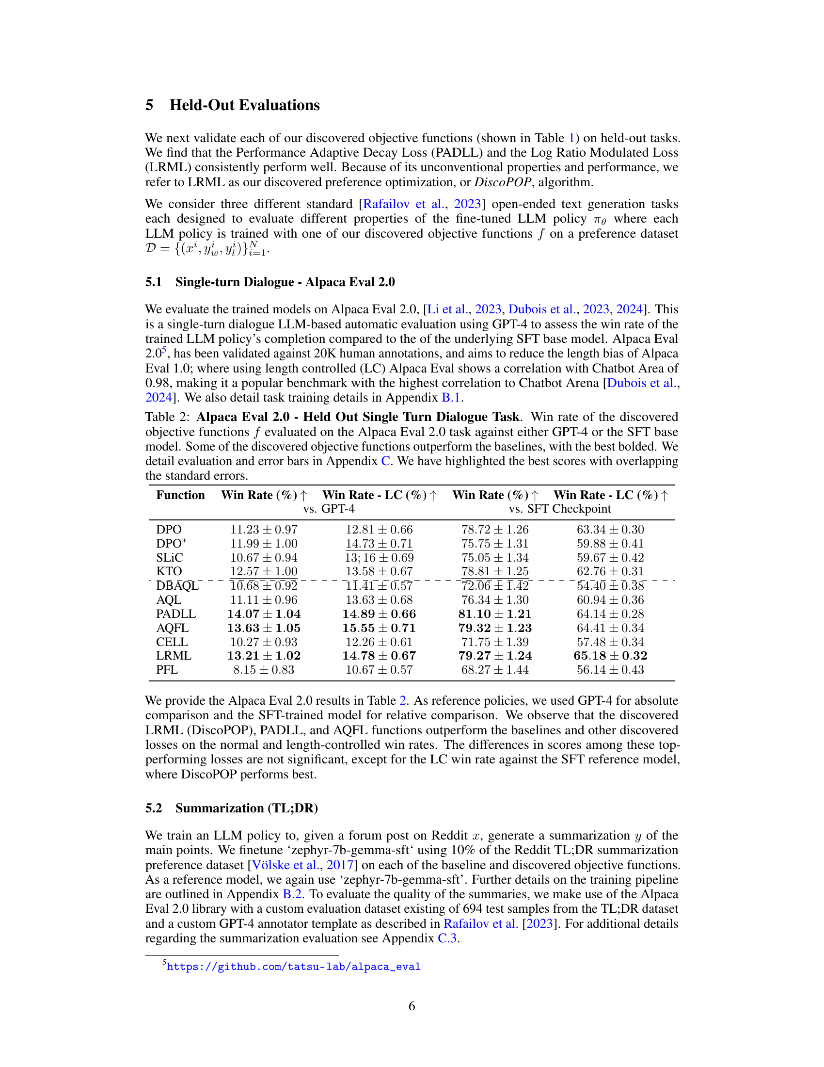
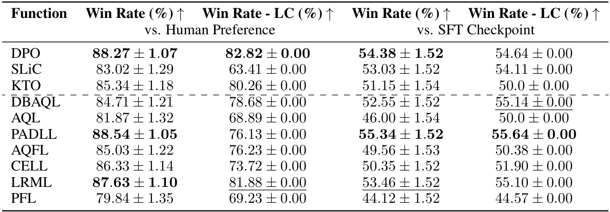
🔼 This table presents the results of evaluating several objective functions (including discovered ones) on the Alpaca Eval 2.0 benchmark for single-turn dialogue. The win rates are calculated against both GPT-4 and the SFT (supervised fine-tuned) base model, with and without length control. The best-performing objective functions are highlighted, taking into account the standard error for statistical significance.
read the caption
Table 2: Alpaca Eval 2.0 - Held Out Single Turn Dialogue Task. Win rate of the discovered objective functions f evaluated on the Alpaca Eval 2.0 task against either GPT-4 or the SFT base model. Some of the discovered objective functions outperform the baselines, with the best bolded. We detail evaluation and error bars in Appendix C. We have highlighted the best scores with overlapping the standard errors.
🔼 This table presents the performance of various objective functions in a multi-turn dialogue task on the MT-Bench benchmark. It lists several baseline objective functions (DPO, SLIC, KTO) followed by the novel objective functions discovered by the LLM-driven method. The scores represent the average performance across different sub-tasks within the MT-Bench evaluation. The table helps to compare the effectiveness of the discovered objective functions against existing state-of-the-art methods.
read the caption
Table 1: Discovery Task MT-Bench Evaluation Scores for each discovered objective function f.

🔼 This table presents the MT-Bench evaluation scores for various objective functions used in offline preference optimization. It compares the performance of several discovered objective functions against established baseline methods (DPO, SLIC, KTO). The table shows the full name, objective function formula, and resulting MT-Bench score for each method. A dashed line separates the baseline methods from the newly discovered ones. More detailed information about each discovered objective function can be found in Appendix E.
read the caption
Table 1: Discovery Task MT-Bench Evaluation Scores for each discovered objective function f. We provide the baselines first, followed by a dashed line to separate the objective functions that were discovered. We provide details for each discovered objective function in Appendix E.

🔼 This table presents the performance of various objective functions (including baselines) on the MT-Bench multi-turn dialogue task. The scores represent the performance of models trained using each objective function. A dashed line separates baseline methods from those discovered using the LLM-driven approach. Details of each discovered objective function are available in Appendix E.
read the caption
Table 1: Discovery Task MT-Bench Evaluation Scores for each discovered objective function f. We provide the baselines first, followed by a dashed line to separate the objective functions that were discovered. We provide details for each discovered objective function in Appendix E.

🔼 This table presents the MT-Bench evaluation scores for various objective functions used in offline preference optimization. It compares the performance of several newly discovered objective functions (listed below the dashed line) against existing baseline methods (above the dashed line). The table includes the full name and mathematical formula for each objective function, allowing for a detailed comparison of their performance on the MT-Bench task. More detailed information about the objective functions is available in Appendix E.
read the caption
Table 1: Discovery Task MT-Bench Evaluation Scores for each discovered objective function f. We provide the baselines first, followed by a dashed line to separate the objective functions that were discovered. We provide details for each discovered objective function in Appendix E.
Full paper#
