TL;DR#
Analyzing the morphology of heartbeats in electrocardiograms (ECGs) is crucial for diagnosing cardiac conditions. However, ECG signals are often corrupted by noise and artifacts, or may be incomplete due to missing leads, presenting challenges for accurate analysis. Existing methods often struggle with these issues. This necessitates robust methods to clean up noisy data and infer complete information from incomplete datasets.
This research proposes BeatDiff, a novel denoising diffusion model, specifically designed to generate high-quality 12-lead ECG heartbeats. They then showcase how BeatDiff can act as a prior for a Bayesian inverse problem, and incorporate it into EM-BeatDiff, an Expectation-Maximization algorithm to solve conditional generation problems. EM-BeatDiff effectively tackles various ECG challenges such as noise and artifact removal, reconstruction of missing leads, and unsupervised anomaly detection, outperforming current state-of-the-art methods.
Key Takeaways#
Why does it matter?#
This paper is important because it introduces a novel method for ECG morphological reconstruction using a lightweight denoising diffusion model, BeatDiff, addressing critical challenges in analyzing heartbeat morphology from noisy or incomplete signals. This has implications for improving cardiac diagnostics and developing new applications for wearable ECG devices. The work bridges generative modeling and Bayesian inverse problems, paving the way for more advanced ECG analysis.
Visual Insights#

🔼 This figure displays two graphs that illustrates the performance of BeatDiff and WGAN in generating ECGs. The left panel shows the ECG generation process along backward diffusion steps. The right panel shows the Earth Mover’s Distance (EMD) between the generated and real ECG distributions for different numbers of diffusion steps. The EMD is used to measure the dissimilarity between probability distributions, lower values indicating greater similarity between the two distributions. This shows that BeatDiff achieves better performance than WGAN across different metrics.
read the caption
Figure 1: Left: heartbeat generation along backward diffusion steps. Right: EMD between generated ECG distribution and real ECG distribution. EMD vs. test (resp. train) in plain (resp. dotted) line. EMD for DDM with different number of diffusion steps, in blue. DDM for WGAN model in gray. EMD between test and train distributions in red. Error bars correspond to different training batches of size 2864.

🔼 This table summarizes the configurations used for EM-BeatDiff in different tasks, including the dimensions of the observation matrix Y (L, T), the unknown parameters θ, the observation matrix Aθ, the artifact matrix Bθ, the noise matrix Dθ, and the noise matrix Dθ. Each row represents a different task with specific parameters.
read the caption
Table 2: Configurations used for EM-BeatDiff for each task.
In-depth insights#
ECG Beat Diffusion#
The concept of “ECG Beat Diffusion” suggests a novel approach to modeling and generating electrocardiogram (ECG) signals. It likely involves using diffusion models, a type of generative AI, to capture the complex, dynamic nature of heartbeats. This approach is particularly promising for handling noisy or incomplete ECG data, common challenges in real-world applications. By training a diffusion model on a large, clean ECG dataset, one could learn a probability distribution representing the underlying patterns of normal heartbeats. This learned distribution then allows the model to generate new, synthetic ECG beats, potentially filling in missing data points or removing noise. Furthermore, a diffusion model’s ability to generate realistic heartbeats could be crucial for applications such as anomaly detection, where deviations from normal patterns indicate potential health problems. However, a careful consideration of model limitations, including potential for generating unrealistic or “hallucinatory” ECG signals, and the ethical implications of using AI-generated medical data, should accompany this promising technique.
Bayesian Inverse Problem#
The concept of a Bayesian inverse problem is central to many areas of science and engineering, especially when dealing with incomplete or noisy data. In this context, the goal is to infer the probability distribution of an unknown parameter or model, given some observed data. Unlike frequentist approaches, the Bayesian approach incorporates prior knowledge or beliefs about the unknown quantity, which is combined with the data likelihood to produce a posterior distribution. This posterior distribution encapsulates all the available information – both prior and data-driven. The Bayesian framework elegantly handles uncertainty inherent in real-world data, allowing for quantification of the uncertainty in the model parameters. The choice of prior distribution can significantly influence the posterior; informative priors can improve estimation accuracy with limited data, while non-informative priors let the data dominate. Computational methods like Markov Chain Monte Carlo (MCMC) or Variational Inference are frequently employed to sample or approximate the posterior distribution, as the posterior is often analytically intractable. The practical effectiveness of the Bayesian inverse problem approach rests on the sensible choice of both prior and likelihood and the selection of an appropriate computational methodology.
EM-BeatDiff Algorithm#
The EM-BeatDiff algorithm cleverly combines a denoising diffusion model (BeatDiff) with a Monte Carlo Expectation-Maximization (MCEM) framework to tackle the challenging problem of ECG heartbeat morphology reconstruction from incomplete or noisy data. BeatDiff acts as a prior, generating realistic ECG beats, while MCEM iteratively refines parameter estimates to best fit the available observations, effectively bridging the gap between the model’s generated data and the measured data. This hybrid approach offers a significant advantage over previous methods: it avoids the need for task-specific fine-tuning and handles various issues inherent to ECG data (missing leads, noise artifacts). The algorithm’s ability to incorporate prior knowledge of the ECG generation process and adapt to different data scenarios makes it robust and versatile, potentially paving the way for improved ECG analysis applications. The integration of BeatDiff and MCEM is a key strength, enabling flexible and accurate reconstruction without retraining for each new task or data condition.
Artifact Removal#
The paper explores artifact removal in ECG signals, a crucial preprocessing step for accurate analysis. The authors frame the problem as a Bayesian inverse problem and leverage their BeatDiff model, a denoising diffusion model, as a prior for improved artifact removal. This approach is particularly valuable because it doesn’t require retraining the model for different artifact types, unlike many traditional methods. EM-BeatDiff, the proposed algorithm, combines BeatDiff with an Expectation-Maximization algorithm to handle unknown model parameters, making it adaptive and robust. The results showcase the method’s effectiveness against baseline wander and electrode motion, with performance surpassing existing state-of-the-art techniques. This method is computationally efficient and offers a flexible framework for various ECG-related tasks, highlighting the potential for real-world applications in improving ECG signal quality. Although the paper uses a Fourier basis for artifact representation, the method itself is flexible and could be adapted with other basis functions. This approach emphasizes the use of generative models as priors in Bayesian inverse problems, which could contribute to advances in many other signal processing applications where artifact removal is a challenge.
Anomaly Detection#
The anomaly detection method proposed leverages a generative model of healthy heartbeats to identify anomalies in ECGs. Instead of directly training a model to classify anomalies, it uses a Bayesian inverse problem framework. This approach reconstructs a healthy version of the input ECG, and the deviation from this reconstruction serves as the anomaly score. The method’s strength lies in its flexibility, as it can handle various types of anomalies and missing data without requiring extensive retraining. By using a pre-trained generative model as a prior, it effectively transfers knowledge from the healthy dataset to the anomaly detection task. This reduces the need for large annotated datasets of abnormal ECGs, a significant limitation in many anomaly detection approaches. The use of the Expectation-Maximization algorithm further enhances the model’s robustness. However, limitations exist, including potential misclassification due to the generative model’s inherent uncertainty and the assumption of a linear inverse model.
More visual insights#
More on figures

🔼 The figure shows the results of using EM-BeatDiff to predict the T-wave based on the QRS complex and heart rate (RR). The left panel shows example predictions for different RR values, while the right panel shows the relationship between the corrected QT interval (QTc) and RR for four patients. The QTc was calculated using both EM-BeatDiff generated data and the Fridericia formula. The results demonstrate the ability of EM-BeatDiff to accurately predict the QTc over a range of RR values, which is essential for diagnosing and managing various cardiac conditions.
read the caption
Figure 2: Left: Example of T-wave prediction (blue) conditioned on Q-wave (red) for different value of RR. Right: QT as a function of RR for 4 patients. QT measured in 100 generated samples (resp. regressed with Fridericia formula) displayed in dots with 95%-CLT bars (resp. curve).

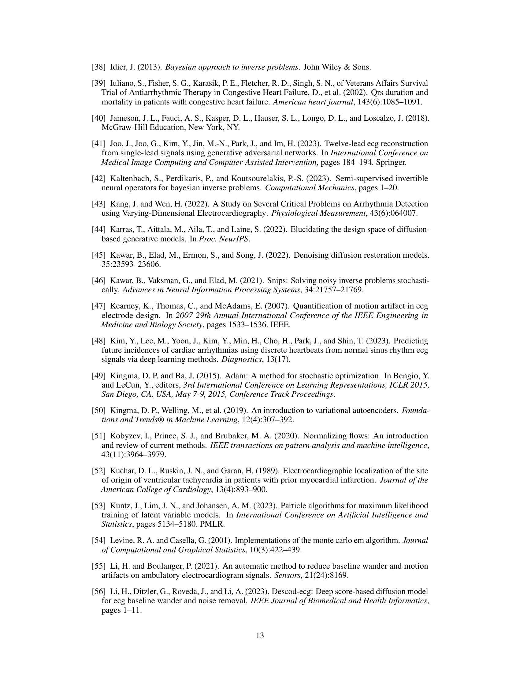
🔼 This figure shows the results of applying EM-BeatDiff and other methods to three tasks: denoising, inpainting, and anomaly detection. The leftmost panel displays an example of a noisy ECG signal. The subsequent panels show the results of denoising with EM-BeatDiff and DeScoD, as well as results obtained with the EM algorithm. The central panels show inpainting results with EM-BeatDiff and EkGAN. The final panel shows anomaly detection results for myocardial infarction (MI) and long QT syndrome (LQT). In all cases, the red ECGs are the actual recordings and the blue ECGs are the results from the corresponding method. The red background highlights the parts of the ECG that were available as input for reconstruction.
read the caption
Figure 3: Illustration of EM-BeatDiff on the denoising, inpaiting and anomaly detection tasks. The red background indicate the parts of the ECG that are observed through y. The red ECGs corresponds to the real ECG and the blue ECGs corresponds to each algorithm reconstructed ECG.

🔼 This figure shows the results of two experiments. The left panel shows the generation of heartbeats along backward diffusion steps. The right panel shows the Earth Mover’s Distance (EMD) between the generated ECG distribution and the real ECG distribution. The EMD is shown for different numbers of diffusion steps and training sets. The figure helps evaluate the quality of generated ECGs by measuring the dissimilarity from real ECG data.
read the caption
Figure 1: Left: heartbeat generation along backward diffusion steps. Right: EMD between generated ECG distribution and real ECG distribution. EMD vs. test (resp. train) in plain (resp. dotted) line. EMD for DDM with different number of diffusion steps, in blue. DDM for WGAN model in gray. EMD between test and train distributions in red. Error bars correspond to different training batches of size 2864.
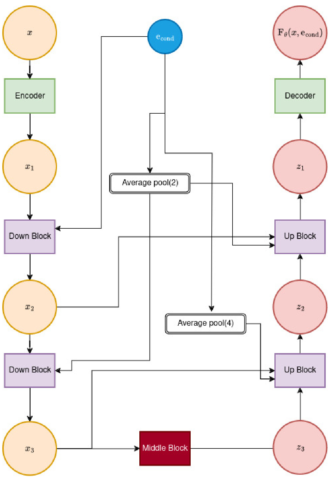
🔼 This figure shows the architecture of the feature extractor network (Fθ) used in BeatDiff. It illustrates a U-Net architecture of depth 2, showing how the input (x, representing the noisy ECG beat) is processed through a series of encoder blocks, average pooling layers, a middle block, and decoder blocks to produce the final output, Fθ(x, econd). The econd vector, combining patient features, time information, and noise level, also feeds into the network. The figure highlights the skip connections and the use of average pooling to reduce the dimensionality of the data.
read the caption
Figure 5: Illustration of Fe architecture for a UNet of depth 2.
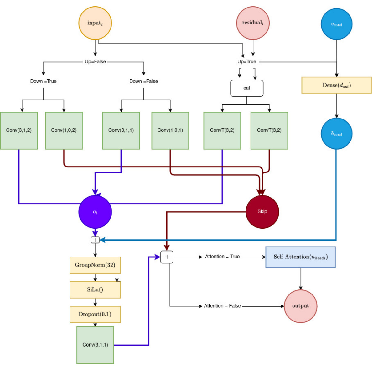
🔼 This figure shows the architecture of a UNet block used in the BeatDiff model. It details the layers and connections within a single block, specifying the use of convolutional layers (Conv), transposed convolutional layers (ConvT), Group Normalization, SiLu activation, dropout, and optional self-attention layers. The parameters Up and Down control whether the block is in the encoder or decoder path of the UNet, dout defines the number of output channels, and Nheads indicates the number of attention heads used if self-attention is enabled. The block uses skip connections to improve information flow through the network.
read the caption
Figure 6: Illustration of a UNet block. Inputs: (Up, Down, dout, Attention, Nheads).
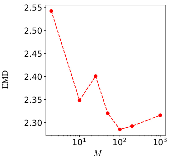
🔼 This figure shows the Earth Mover’s Distance (EMD) between 1000 samples generated using the Sequential Monte Carlo (SMC) algorithm with varying numbers of particles (M) and 1000 samples generated with a large number of particles (M=105). The EMD serves as a measure of the dissimilarity between the generated sample distribution and a reference distribution. The plot shows that as the number of particles increases, the EMD decreases, indicating that the generated sample distribution converges towards the reference distribution. The optimal number of particles M that balances computational cost and accuracy is discussed in the text.
read the caption
Figure 7: EMD distance between 1000 samples from algorithm 1 with M particles and 1000 samples of algorithm 1 with 105 particles, that is considered the standard samples.

🔼 This figure compares the performance of the proposed DDM (BeatDiff) model against a WGAN model in generating ECG heartbeats. It displays six examples of real ECGs alongside their corresponding reconstructions generated by each model. The visual comparison allows for a qualitative assessment of how well each model captures the characteristics of real ECG data, such as the shape and amplitude of various waves and segments.
read the caption
Figure 9: Real and generated ECG heart beat with DDM and WGAN.
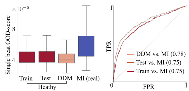
🔼 The figure presents a comparison of the out-of-distribution (OOD) scores for four different groups: training data, testing data, generated ECG beats from BeatDiff, and real ECG beats from patients diagnosed with myocardial infarction (MI). The left panel shows box plots visualizing the distribution of OOD scores for each group. The right panel displays receiver operating characteristic (ROC) curves, illustrating the performance of a classifier in distinguishing MI ECGs from the other three groups using the OOD score as a feature.
read the caption
Figure 8: Out-of-distribution evaluation. Left. Box-plot of OOD-score for train, test, generated (Gen) and MI heart beats. Right. ROC curves for classification between train/test/gen and MI based on OOD-score.
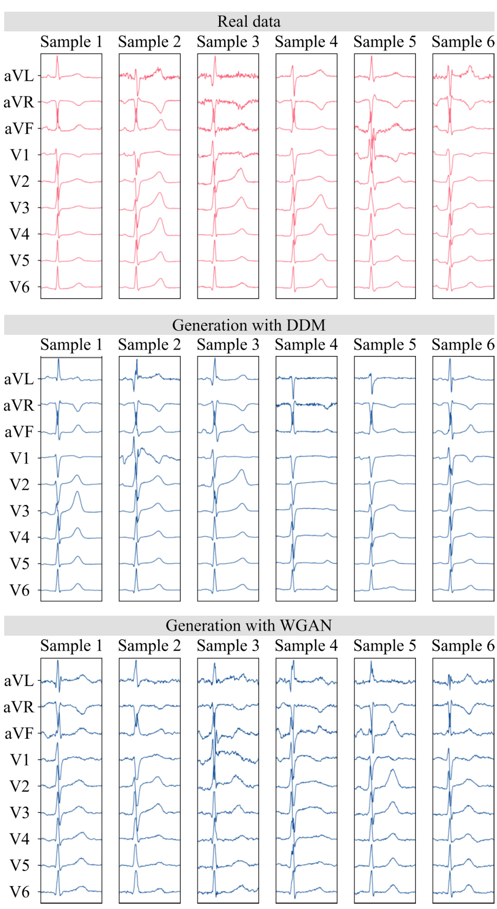
🔼 This figure compares the quality of ECG heartbeats generated by different models. The top panel shows six real ECG heartbeats, while the middle and bottom panels display six synthetic ECGs generated using a diffusion model and a Generative Adversarial Network (GAN), respectively. The visualization allows for a visual comparison of the models’ performance in generating realistic heartbeats.
read the caption
Figure 9: Real and generated ECG heart beat with DDM and WGAN.
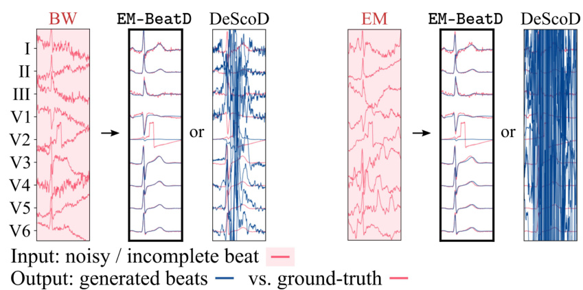
🔼 This figure shows a comparison of EM-BeatDiff with other methods (DeScoD and EkGAN) for three different tasks: denoising, inpainting, and anomaly detection. For each task, the leftmost panel shows the noisy or incomplete input ECG, while the subsequent panels illustrate the results obtained by each method. The red lines represent the ground truth ECG, whereas the blue lines depict the ECGs reconstructed by the respective algorithms. Red backgrounds in the ECG segments indicate the portions observed through y during reconstruction.
read the caption
Figure 3: Illustration of EM-BeatDiff on the denoising, inpaiting and anomaly detection tasks. The red background indicate the parts of the ECG that are observed through y. The red ECGs corresponds to the real ECG and the blue ECGs corresponds to each algorithm reconstructed ECG.

🔼 This figure compares the performance of a diffusion model (DDM) and a Wasserstein Generative Adversarial Network (WGAN) in generating ECG heartbeats. The top panel shows six real ECG beats from the dataset. The middle panel shows six ECG beats generated using the DDM, and the bottom panel shows six ECG beats generated using the WGAN. The figure visually demonstrates the ability of the DDM to generate more realistic ECG signals compared to the WGAN.
read the caption
Figure 9: Real and generated ECG heart beat with DDM and WGAN.

🔼 This figure compares the performance of the proposed Denoising Diffusion Model (DDM) with a Wasserstein Generative Adversarial Network (WGAN) for generating ECG heartbeats. It displays six samples each of real ECG data, ECGs generated using the DDM, and ECGs generated using the WGAN, all shown across the standard 12 leads. The goal is to visually assess the quality and realism of the generated ECGs compared to real ECG recordings.
read the caption
Figure 9: Real and generated ECG heart beat with DDM and WGAN.
More on tables

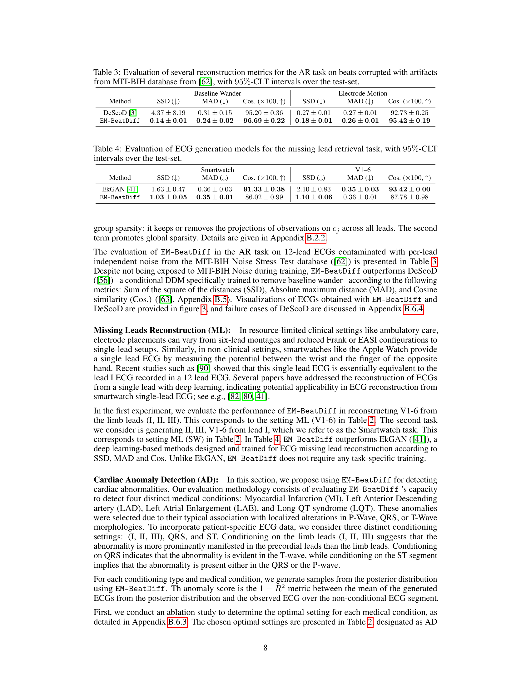
🔼 This table presents the performance comparison of DeScoD and EM-BeatDiff on artifact removal tasks using three evaluation metrics: Sum of Squared Deviations (SSD), Maximum Absolute Deviation (MAD), and Cosine Similarity (Cos). Lower SSD and MAD values and higher Cosine similarity indicate better performance. The results are shown separately for baseline wander and electrode motion artifacts, and 95% confidence intervals are provided.
read the caption
Table 3: Evaluation of several reconstruction metrics for the AR task on beats corrupted with artifacts from MIT-BIH database from [62], with 95%-CLT intervals over the test-set.

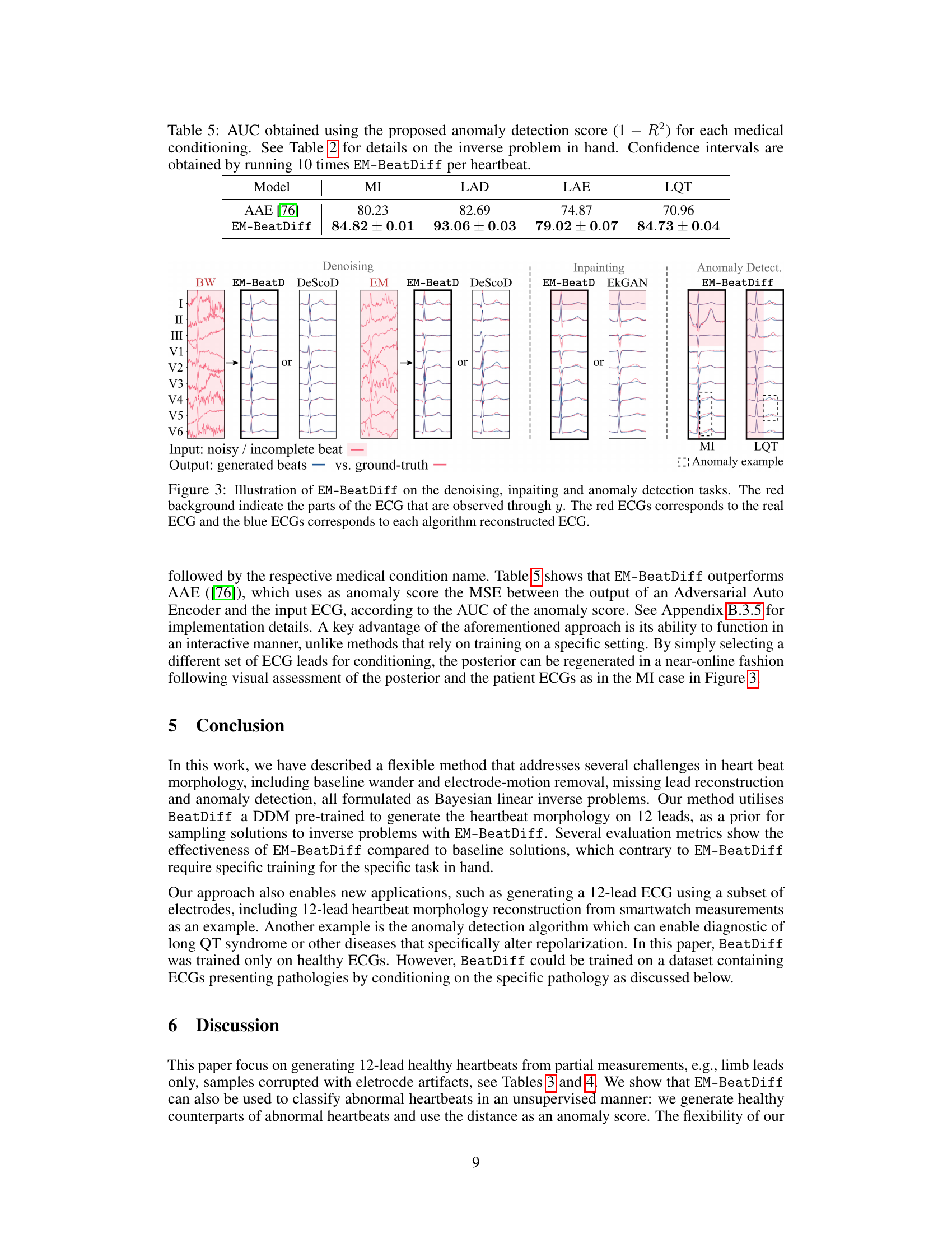
🔼 This table presents the quantitative results of evaluating different ECG generation models on the task of reconstructing missing leads. The models were evaluated using three metrics: Sum of Squared Differences (SSD), Mean Absolute Deviation (MAD), and Cosine Similarity (Cos). Lower values for SSD and MAD indicate better performance, while higher cosine similarity values represent a better match to the original ECG. The results are shown for two scenarios: reconstructing leads V1-V6 from leads I, II, III, and reconstructing all leads from only lead I (simulating a smartwatch scenario). 95% confidence intervals are provided for each metric, reflecting the uncertainty in the model performance.
read the caption
Table 4: Evaluation of ECG generation models for the missing lead retrieval task, with 95%-CLT intervals over the test-set.

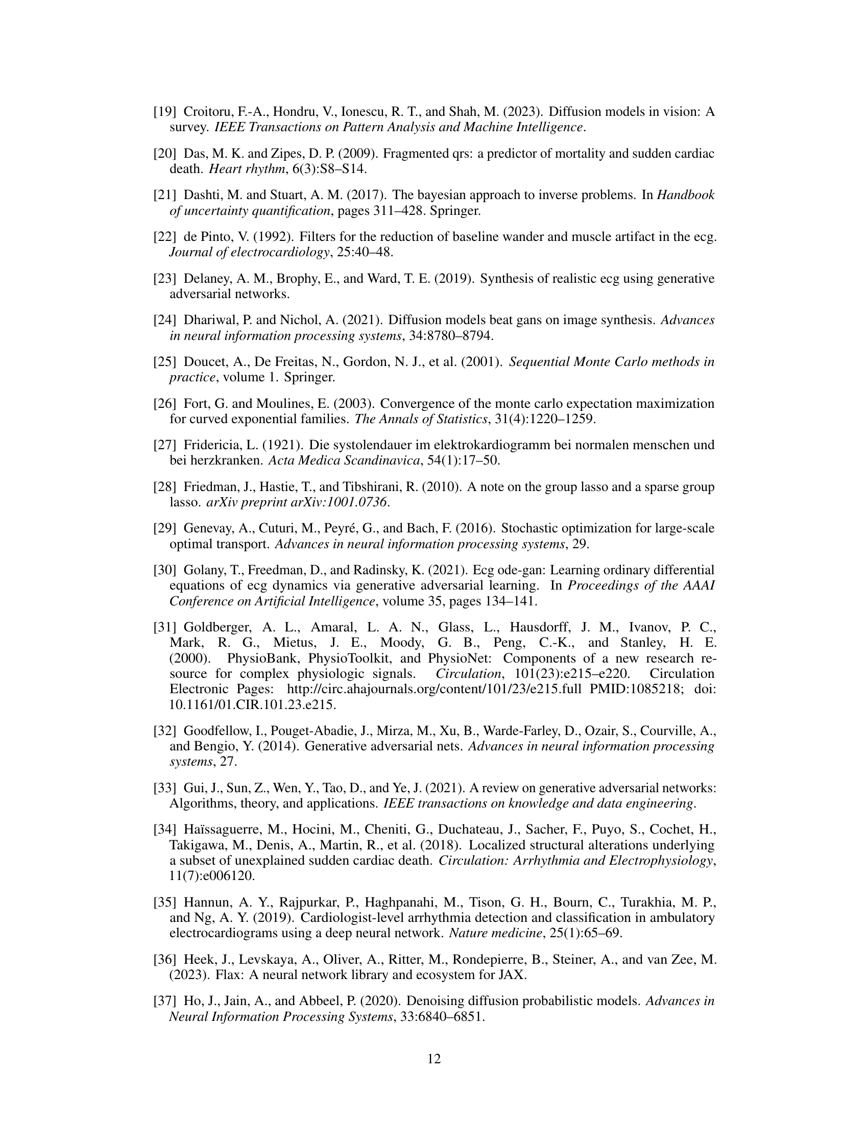
🔼 This table presents the Area Under the Curve (AUC) scores for the anomaly detection task using the proposed EM-BeatDiff method. The AUC is calculated using the (1-R^2) metric, comparing the mean of generated ECGs to the observed ECGs for each of four medical conditions (MI, LAD, LAE, LQT). Different conditioning strategies (I,II,III, QRS, ST) are used, based on the availability of ECG segments. Confidence intervals are provided to show statistical significance.
read the caption
Table 5: AUC obtained using the proposed anomaly detection score (1 – R2) for each medical conditioning. See Table 2 for details on the inverse problem in hand. Confidence intervals are obtained by running 10 times EM-BeatDiff per heartbeat.

🔼 This table compares the performance of several ECG generation models in a heartbeat sex classification task. The task uses an imbalanced dataset where the number of female heartbeats (F) is significantly smaller than the number of male heartbeats (M). The models are used to balance the dataset by generating additional female heartbeats. The table presents the model size, inference time, F1 score, accuracy, and AUC (Area Under the Curve) for two different levels of imbalance (F=10%M and F=5%M). Confidence intervals are included to show the reliability of the results.
read the caption
Table 1: Evaluation of ECG generation models for balancing sex-imbalanced datasets in heartbeat classification task. F and M refer to the number of female and male real heartbeats in the training set. Confidence intervals are obtained by re-initializing the classifier training and the generated data used to balance the datasets.

🔼 This table presents the performance comparison of various ECG generation models in a heartbeat classification task. The models were used to balance a sex-imbalanced dataset, which involved generating additional data for the under-represented sex (female in this case). The table shows the model size, inference time, F1-score, accuracy, and AUC for different ratios of female to male heartbeats. The results show that BeatDiff outperforms the other models across all metrics.
read the caption
Table 1: Evaluation of ECG generation models for balancing sex-imbalanced datasets in heartbeat classification task. F and M refer to the number of female and male real heartbeats in the training set. Confidence intervals are obtained by re-initializing the classifier training and the generated data used to balance the datasets.

🔼 This table compares the performance of several ECG generation models in a heartbeat sex classification task. The models are evaluated on their ability to balance an imbalanced dataset by generating synthetic data for the underrepresented sex. Metrics include F1 score, accuracy, and AUC, and confidence intervals are reported to account for variability in model training. The table also notes the model size and inference time. The goal is to assess which models improve classification performance best by generating realistic ECGs for underrepresented cases.
read the caption
Table 1: Evaluation of ECG generation models for balancing sex-imbalanced datasets in heartbeat classification task. F and M refer to the number of female and male real heartbeats in the training set. Confidence intervals are obtained by re-initializing the classifier training and the generated data used to balance the datasets.

🔼 This table shows the configuration of a deeper network architecture that was tested. It provides details on the parameters used for different layers of the network, including the output dimensions for each layer. This deeper network was an alternative architecture explored in the study.
read the caption
Table 8: Configuration of deeper network tested.
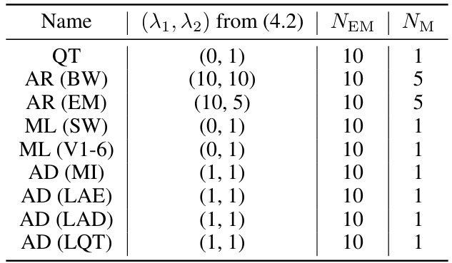
🔼 This table lists the hyperparameters used in the EM algorithm within EM-BeatDiff for different tasks. Specifically, it shows the regularization parameters (λ₁, λ₂) from equation (4.2), the total number of EM steps (NEM), and the number of gradient steps per M-step (NM) for each task (QT, Artifact Removal (baseline wander and electrode motion), Missing Leads Reconstruction (from a single lead and V1-6 leads), and Anomaly Detection for several cardiac anomalies). These parameters influence the optimization process within the EM algorithm.
read the caption
Table 9: Parameters used fo EM-BeatDiff.
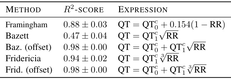
🔼 This table presents the R-squared scores resulting from regressing different corrected QT formulas against the QT interval obtained from generated ECG beats. The formulas used are Framingham, Bazett, Bazett with offset, Fridericia, and Fridericia with offset. The R-squared values represent the goodness of fit of each formula in predicting the QT interval based on the RR interval. The 95% confidence intervals are also provided.
read the caption
Table 10: R2-score between QT measured vs. regressed (intercept: QT, slope: QT₁) as a function of RR, in generated samples, with 95%-CLT intervals over the test-set.

🔼 This table shows the configurations used in the ablation study for cardiac anomaly detection. Different configurations represent different ways of conditioning the model (using different subsets of leads or segments of the ECG signal). The configurations are described in terms of the dimensions of matrices involved in the Bayesian inverse problem, as well as the values of several hyperparameters.
read the caption
Table 11: Configurations tested in the ablation study.

🔼 This table presents the Area Under the Curve (AUC) scores for anomaly detection of four different cardiac conditions (MI, LAD, LAE, LQT) using the EM-BeatDiff method. The AUC scores are calculated using three different conditioning strategies: (I, II, III) uses only the limb leads for conditioning, QRS conditions on the QRS complex, and ST conditions on the ST segment. Confidence intervals are provided for each result, reflecting the variability inherent in the EM-BeatDiff method.
read the caption
Table 12: Anomaly detection abblation study. Confidence intervals are obtained by running 10 times EM-BeatDiff per heartbeat.
Full paper#

