TL;DR#
Diffusion models are powerful generative models, but controlling their output remains challenging. Existing methods like classifier guidance require additional training, limiting their flexibility and applicability. Training-free guidance offers a promising alternative by using pretrained networks, achieving zero-shot conditional generation. However, this approach has limitations such as misaligned gradients and slower convergence.
This paper delves into the theoretical underpinnings of training-free guidance, revealing its susceptibility to misaligned gradients and slower convergence compared to classifier-based methods. To overcome these limitations, the authors introduce random augmentation to enhance gradient alignment and a Polyak step size schedule to improve convergence rates. Extensive experiments across different diffusion models and various control conditions (image and motion generation) validate the effectiveness of these proposed techniques, demonstrating significant improvements in both quality and efficiency.
Key Takeaways#
Why does it matter?#
This paper is crucial because it tackles the limitations of training-free guidance in diffusion models, a rapidly growing area of research. By offering theoretical insights and practical solutions, it paves the way for more robust and efficient controlled generation in various applications. The improved techniques presented directly address current challenges, making training-free guidance more reliable and applicable. This work is relevant for researchers working on diffusion models, generative AI, and related fields.
Visual Insights#

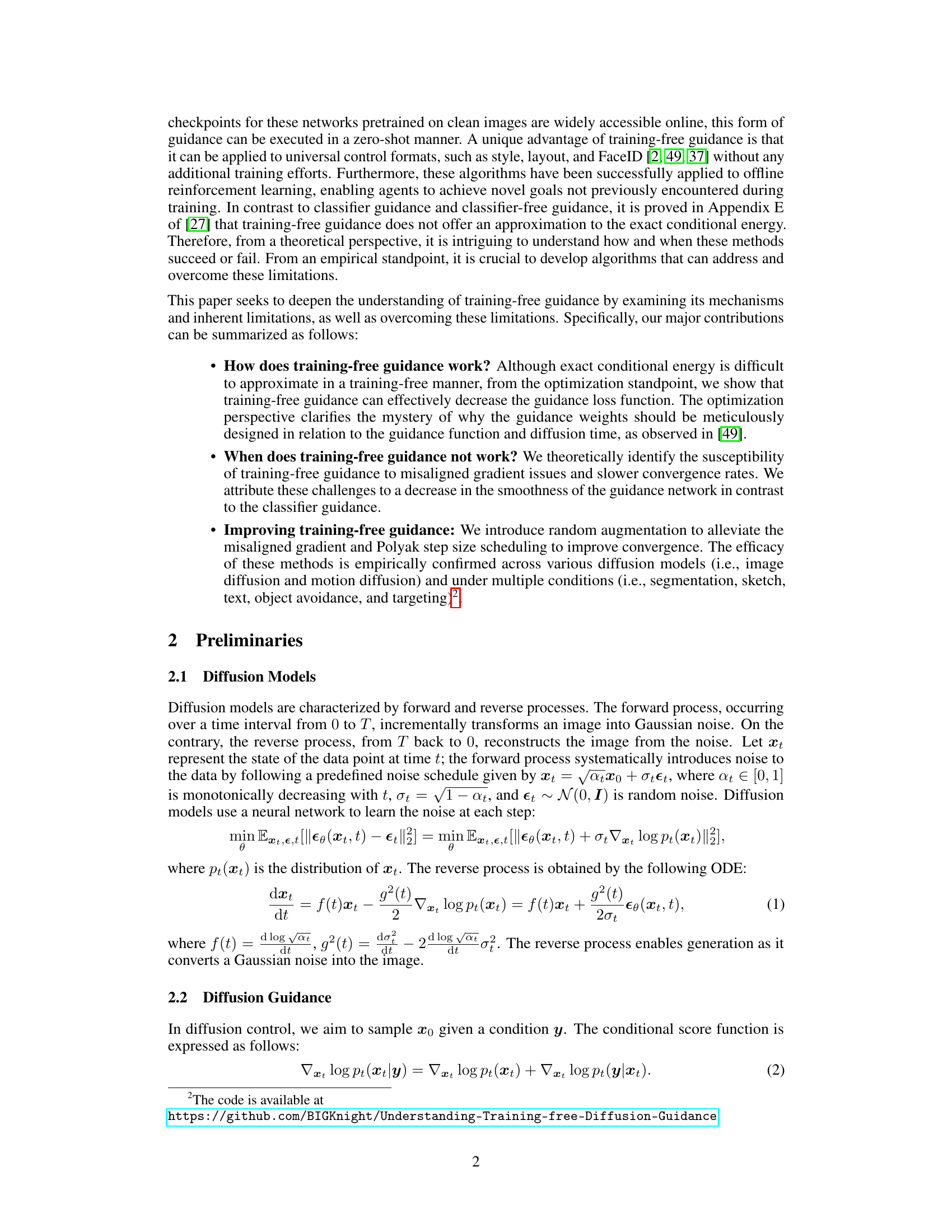
🔼 This figure shows two examples of training-free guidance, one successful and one unsuccessful. The successful example shows a smooth decrease in the loss function over diffusion time, indicating effective guidance towards the target class. Conversely, the unsuccessful example shows oscillations and minimal loss reduction despite the absence of the target class, revealing issues with misaligned gradients. The target class for both examples is ‘indigo bird’.
read the caption
Figure 1: The classifier loss of a successful and a failure guidance example. The target class is 'indigo bird'.

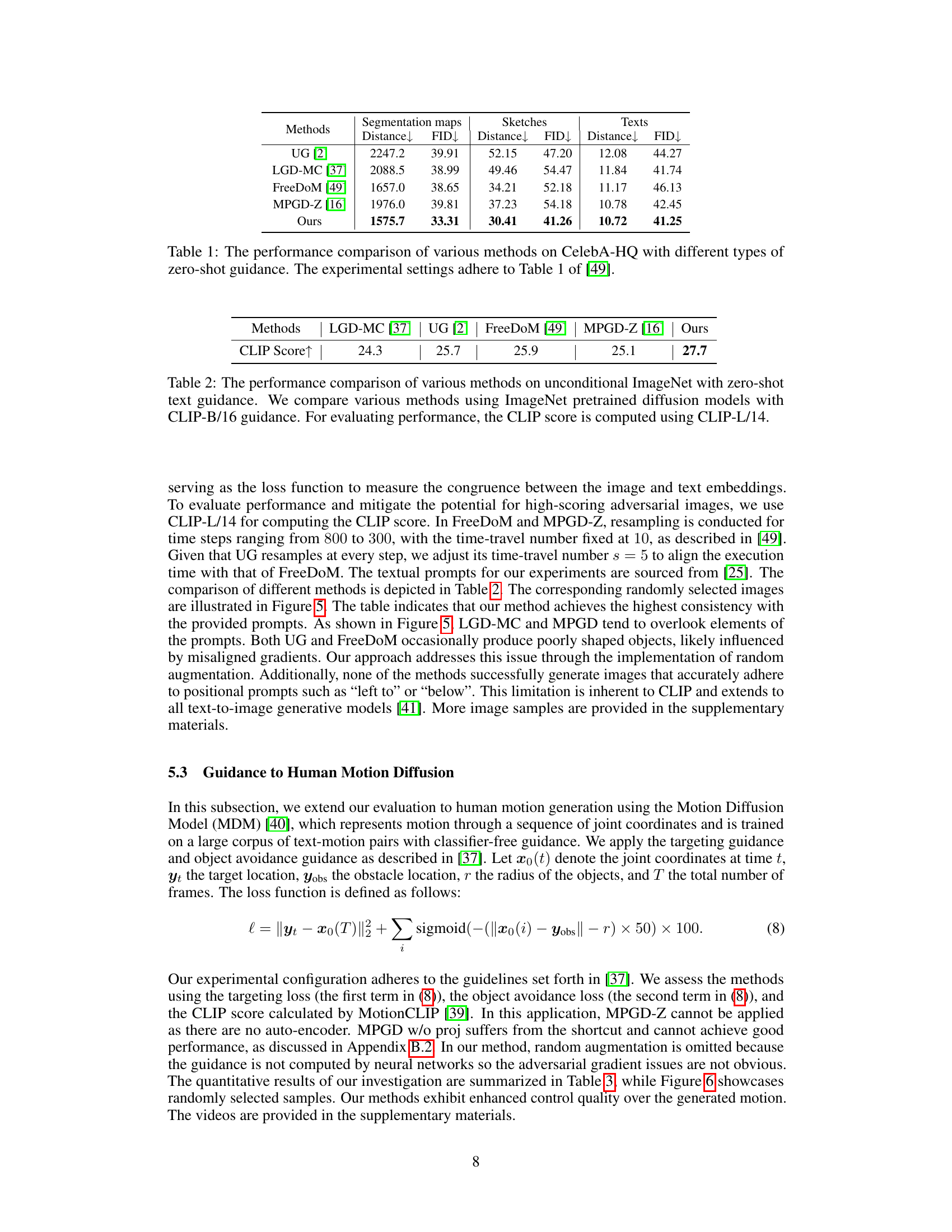
🔼 This table compares the performance of different methods on the CelebA-HQ dataset using three different types of zero-shot guidance: segmentation maps, sketches, and text descriptions. The results are presented in terms of FID (Fréchet Inception Distance) and a distance metric. Lower FID and distance values indicate better performance. The experimental setup mirrors that of a previous study [49] for fair comparison.
read the caption
Table 1: The performance comparison of various methods on CelebA-HQ with different types of zero-shot guidance. The experimental settings adhere to Table 1 of [49].
In-depth insights#
Training-Free Limits#
The concept of “Training-Free Limits” in the context of diffusion models highlights the inherent trade-offs and challenges associated with achieving effective guidance without explicit training. While training-free methods offer the appealing benefit of zero-shot capability and broad applicability, they are fundamentally limited by their reliance on pretrained networks designed for clean data. This reliance introduces several constraints: Misaligned gradients, where the guidance network’s optimization direction deviates from the desired trajectory; slower convergence rates, compared to classifier-based approaches, stemming from the reduced smoothness of the guidance network; and inadequate approximation of the true conditional energy, leading to potential instability and suboptimal results. Addressing these limits necessitates novel techniques to improve gradient alignment, accelerate convergence, and potentially explore alternative estimation methods for the conditional energy. The exploration of “Training-Free Limits” thus becomes a crucial area of research for unlocking the full potential of training-free diffusion guidance while mitigating its inherent weaknesses.
Gradient Misalignment#
Gradient misalignment in training-free diffusion guidance is a critical issue stemming from the discrepancy between the gradients of the pretrained network (used for guidance) and the true conditional energy of the diffusion process. The pretrained network, optimized for clean images, doesn’t perfectly capture the noisy image landscape, leading to gradients that aren’t optimally aligned with the desired generative direction. This results in slower convergence and suboptimal sample quality; the model struggles to accurately incorporate the desired conditions, leading to misaligned or distorted outputs. Addressing this challenge requires methods that either improve the alignment of gradients (e.g., time-dependent classifiers or adding noise) or mitigate the effects of misalignment (e.g., random augmentation, Polyak step size scheduling). The theoretical analysis highlighting the susceptibility of training-free guidance to misaligned gradients provides a framework for understanding the limitations of this approach and inspires the development of improved training-free methods. The success of techniques like random augmentation empirically demonstrates the importance of addressing gradient misalignment for better control and quality in diffusion models.
Augmentation Effects#
Data augmentation, the process of artificially enhancing datasets to improve model robustness and generalization, plays a crucial role in deep learning. In the context of diffusion models, augmentation’s impact on guidance mechanisms is particularly significant. Applying augmentations to noisy input data before feeding it to a guidance network, for example, can influence the gradient calculations and subsequent adjustments made during the diffusion process. This impact can manifest as a reduction in misaligned gradients, thereby improving the efficiency of the guidance and the quality of generated samples. The choice of augmentation strategy is crucial, as it must not introduce unwanted artifacts or distort the fundamental information embedded in the noisy input. The effectiveness of augmentation often depends on factors like the choice of the underlying diffusion model, the specific augmentation techniques used, and how the augmentations interact with the guidance network architecture. Careful selection and parameter tuning are crucial for optimal results, particularly for high-dimensional data like images and videos, where uncontrolled augmentation can hinder the convergence and lead to unintended consequences.
Convergence Rates#
Analyzing convergence rates in machine learning models is crucial for evaluating efficiency and performance. Faster convergence generally implies reduced training time and computational cost. However, the rate at which a model converges can be significantly impacted by various factors, including the model architecture, the optimization algorithm employed, the dataset characteristics (e.g., size, dimensionality, noise), and the initialization strategy. Understanding these factors is essential for developing effective training strategies. Theoretical analyses often provide insights into the upper bounds on convergence rates, while empirical studies offer practical guidance based on real-world experiments. A key aspect of convergence analysis is assessing the stability of the process; a slow or erratic convergence might indicate instability and challenges in achieving a globally optimal solution. Therefore, a comprehensive study of convergence rates involves both theoretical underpinnings and experimental validation, carefully considering the interplay between model properties and training methodologies to optimize the learning process.
Future Directions#
Future research could explore several promising avenues. Improving the efficiency of training-free guidance is crucial, perhaps by developing more sophisticated optimization techniques or exploring alternative network architectures. Addressing the misaligned gradient issue is also vital; this could involve incorporating techniques from adversarial training or developing new regularization methods. A deeper understanding of the relationship between training-free guidance and the convergence rate of the reverse diffusion process is needed, possibly through a more thorough theoretical analysis. Investigating the applicability of training-free guidance to other generative models beyond diffusion models would broaden its impact. Finally, extending training-free guidance to more complex tasks such as video generation and 3D modeling would be a significant step forward. These research directions have the potential to unlock the full power of training-free guidance and broaden its use in diverse applications.
More visual insights#
More on figures

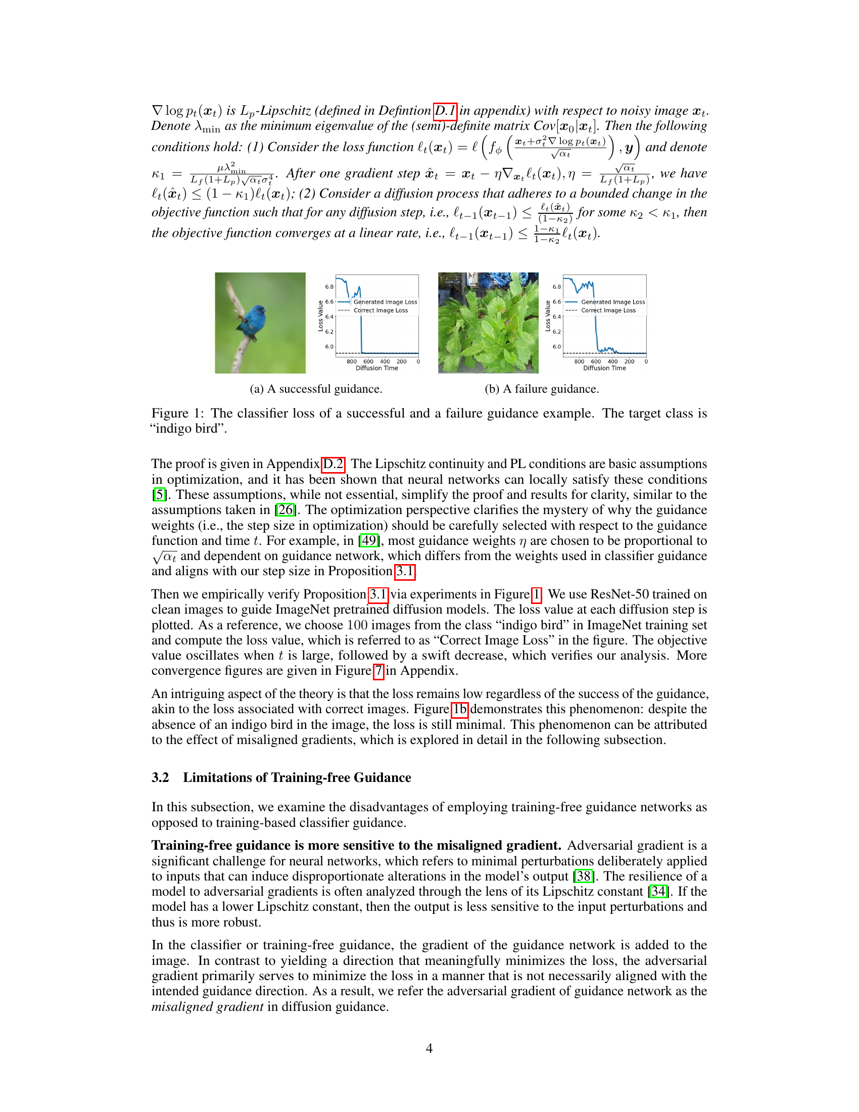
🔼 This figure compares the gradients produced by different classifiers when applied to random background images. The top row shows the target image class ‘cock’, while the bottom row shows the target image class ‘goldfinch’. Four different classifier types are shown: (a) an adversarially robust classifier; (b) a time-dependent classifier; (c) an off-the-shelf ResNet-50 classifier; and (d) a ResNet-50 classifier with random augmentation. The visualization demonstrates how the type of classifier affects the gradient’s clarity and alignment with the target image, highlighting the impact of time-dependence and augmentation on robustness to misaligned gradients.
read the caption
Figure 2: Gradients of different classifiers on random backgrounds. The images in the first row correspond to the target class “cock”, and the second row to “goldfinch”.

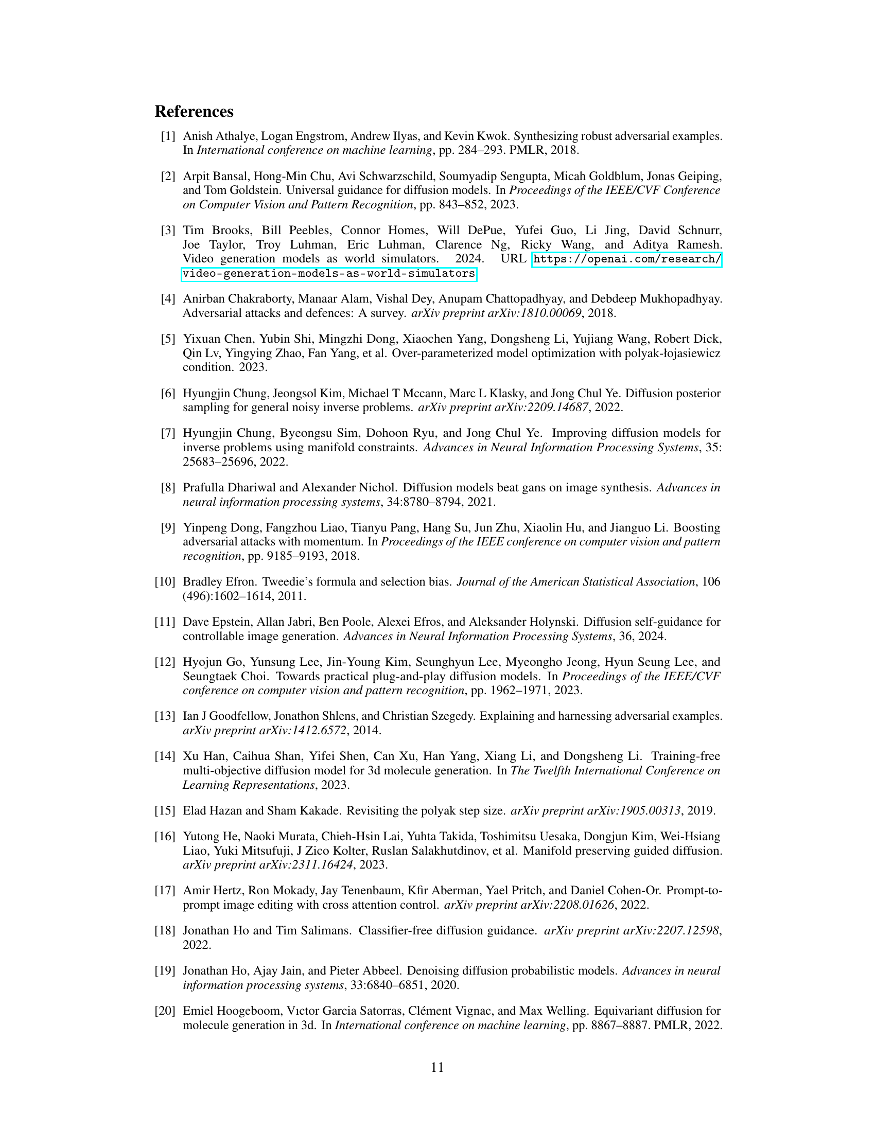
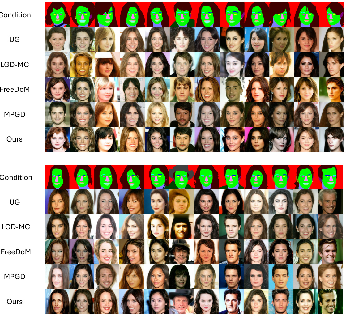
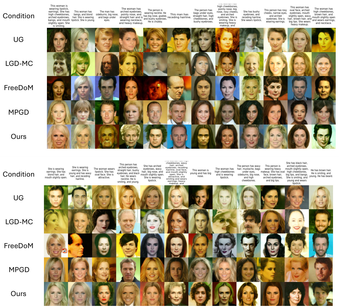
🔼 This figure displays the qualitative results of applying three different types of zero-shot guidance (segmentation, sketch, and text) to a CelebA-HQ diffusion model. Each row represents a different guidance method (UG, LGD-MC, FreeDoM, MPGD, and the authors’ method), and each column shows the generated images from a different seed. The images are randomly selected to showcase the visual quality and diversity of the generated samples under each guidance condition.
read the caption
Figure 4: Qualitative results of CelebA-HQ with zero-shot segmentation, sketch, and text guidance. The images are randomly selected.
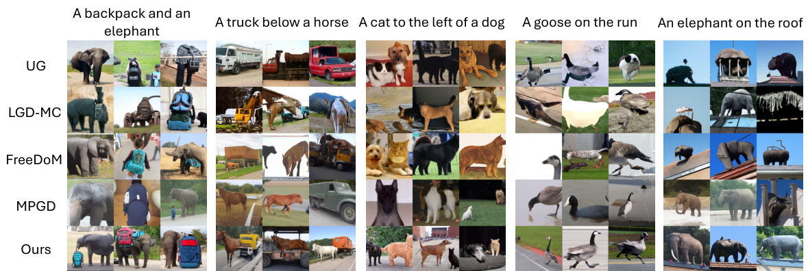
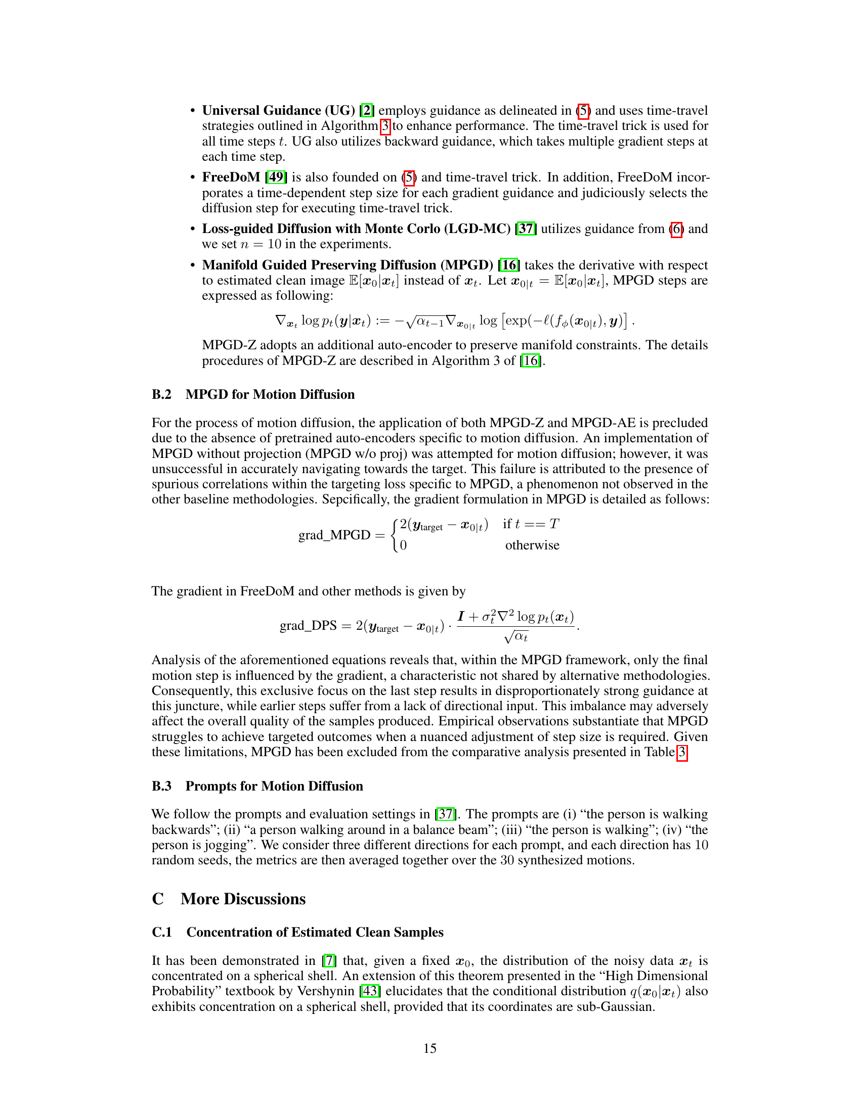
🔼 This figure shows the qualitative results of applying zero-shot text guidance to an ImageNet pretrained diffusion model. Different methods (UG, LGD-MC, FreeDoM, MPGD, and the proposed ‘Ours’) are compared. Each row corresponds to a different method, and each column displays generated images for a specific text prompt. The prompts represent various scene descriptions, including animals, objects and landscapes. The images generated demonstrate the effectiveness of each method in fulfilling the specified text prompts. Randomly selected images are shown for each method and prompt.
read the caption
Figure 5: Qualitative results of ImageNet model with zero-shot text guidance. The images are randomly selected.
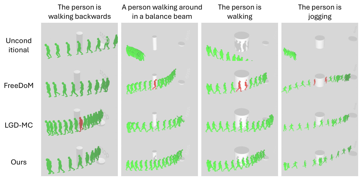
🔼 This figure shows a comparison of different methods for human motion generation with zero-shot object avoidance and targeting guidance. Four different motion types are demonstrated (walking backward, walking on a balance beam, walking, and jogging). Each method (Unconditional, FreeDoM, LGD-MC, and Ours) is shown generating motion sequences for each motion type. The presence of obstacles and their avoidance are also highlighted. The key difference between these methods should be observable in how well the methods manage to navigate obstacles and accurately perform the desired motion.
read the caption
Figure 6: Qualitative results of human motion diffusion with zero-shot object avoidance and targeting guidance. Instances of intersection with obstacles are highlighted by marking the person in red. The trajectories are randomly selected.
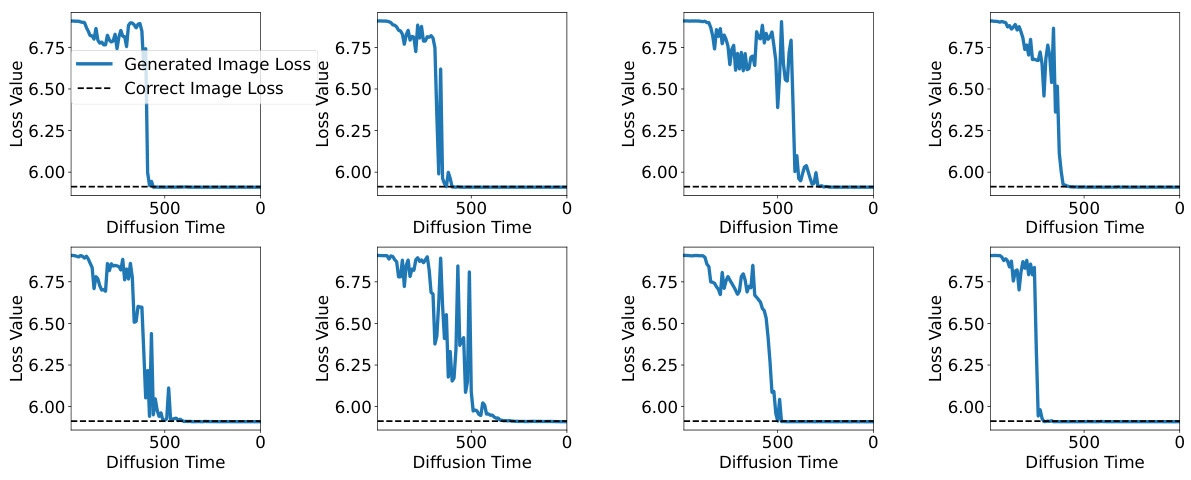
🔼 This figure shows the classifier loss curves for two examples of training-free guidance in a diffusion model. The target class is ‘indigo bird’. The left panel (a) shows a successful guidance example, where the loss steadily decreases as the diffusion process progresses (t decreases from 800 to 0). The right panel (b) depicts a failed guidance, where the loss remains consistently low, even though the generated image doesn’t contain the target class. The figure illustrates how training-free guidance can sometimes fail to effectively guide the diffusion process toward generating a desired image.
read the caption
Figure 1: The classifier loss of a successful and a failure guidance example. The target class is 'indigo bird'.
🔼 This figure shows a qualitative comparison of gradients generated by different classifiers on random backgrounds. The top row shows the target image, “cock”, while the bottom row shows the target image “goldfinch”. Each column represents a different classifier: (a) adversarially robust classifier; (b) time-dependent classifier; (c) off-the-shelf ResNet-50 classifier; and (d) ResNet-50 classifier with random augmentation. The visualization demonstrates how the accumulated gradients from different classifiers vary, highlighting the impact of classifier type on gradient quality and alignment with the target image. This is used to support the paper’s analysis on the misaligned gradients found in training-free guidance.
read the caption
Figure 2: Gradients of different classifiers on random backgrounds. The images in the first row correspond to the target class “cock”, and the second row to “goldfinch”.

🔼 This figure shows a qualitative comparison of gradients generated by different classifiers on random backgrounds. The top row displays target images of ‘cock’, and the bottom row shows target images of ‘goldfinch’. Each column represents the accumulated gradient for a different classifier: Adversarially robust classifier, time-dependent classifier, off-the-shelf ResNet-50 classifier, and ResNet-50 classifier with random augmentation. The visualization aims to highlight the effect of different classifier types on gradient quality and alignment with the target image, indicating the susceptibility of off-the-shelf classifiers to misaligned gradients.
read the caption
Figure 2: Gradients of different classifiers on random backgrounds. The images in the first row correspond to the target class “cock”, and the second row to “goldfinch”.
🔼 This figure compares the gradients generated by different types of classifiers when applied to random backgrounds. It visually demonstrates the impact of different classifier architectures on the quality and alignment of the resulting gradients. The first row showcases the target class ‘cock’, while the second row displays the target class ‘goldfinch’. By comparing the gradients, one can assess the effectiveness and robustness of each classifier in guiding the diffusion process.
read the caption
Figure 2: Gradients of different classifiers on random backgrounds. The images in the first row correspond to the target class “cock”, and the second row to “goldfinch”.

🔼 This figure presents a qualitative comparison of gradients generated by different types of classifiers on random backgrounds. The goal is to show how the accumulated gradients, when used for guidance in diffusion models, vary in their visual resemblance to the target image. The classifiers compared are an adversarially robust classifier, a time-dependent classifier, and an off-the-shelf ResNet-50 classifier, both with and without random augmentation. The image in the first row of each block is the target class for comparison. The comparison aims to highlight the tendency of off-the-shelf classifiers (without time-dependence or augmentation) to produce misaligned gradients that hinder effective guidance compared to their time-dependent counterparts.
read the caption
Figure 2: Gradients of different classifiers on random backgrounds. The images in the first row correspond to the target class “cock”, and the second row to “goldfinch”.
More on tables

🔼 This table compares the performance of different methods for generating CelebA-HQ images under three zero-shot guidance conditions: segmentation maps, sketches, and text descriptions. The metrics used are FID (Fréchet Inception Distance) and Distance (a custom distance metric specified in the paper). Lower FID and Distance scores indicate better image quality and alignment with the guidance, respectively. The methods compared include Universal Guidance (UG), Loss-Guided Diffusion with Monte Carlo (LGD-MC), Training-Free Energy-Guided Diffusion Models (FreeDoM), Manifold Preserving Guided Diffusion (MPGD-Z), and the proposed method in the paper. The experimental setup mirrors Table 1 from the cited reference [49].
read the caption
Table 1: The performance comparison of various methods on CelebA-HQ with different types of zero-shot guidance. The experimental settings adhere to Table 1 of [49].

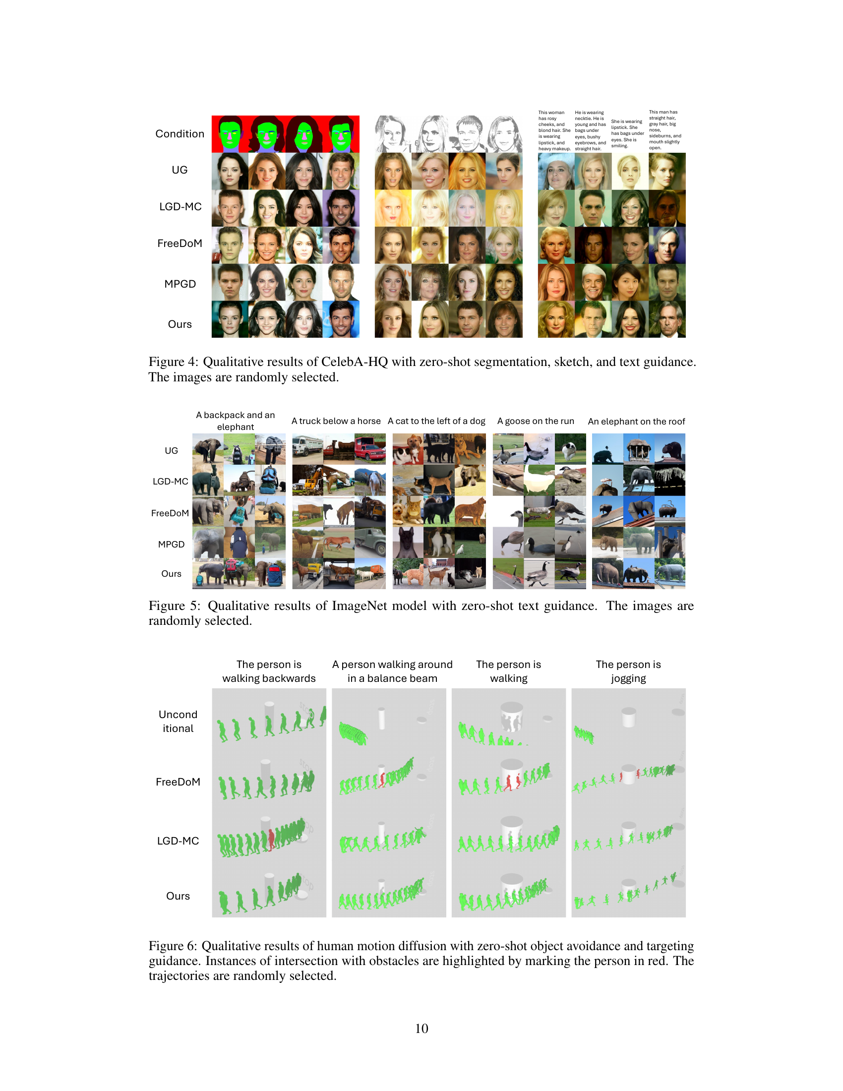
🔼 This table compares the performance of different training-free guidance methods on unconditional ImageNet generation using zero-shot text guidance. The methods are evaluated using CLIP-B/16 for guidance and CLIP-L/14 for scoring, providing a measure of how well the generated images align with the input text prompts. Higher CLIP scores indicate better alignment.
read the caption
Table 2: The performance comparison of various methods on unconditional ImageNet with zero-shot text guidance. We compare various methods using ImageNet pretrained diffusion models with CLIP-B/16 guidance. For evaluating performance, the CLIP score is computed using CLIP-L/14.

🔼 This table compares different methods for human motion generation using the Motion Diffusion Model (MDM). It evaluates performance on zero-shot targeting and object avoidance tasks. The loss is a combined measure of the Mean Squared Error (MSE) between the target and final position, and an object avoidance loss. The CLIP score is also included as another metric of performance.
read the caption
Table 3: Comparison of various methods on MDM with zero-shot targeting and object avoidance guidance. Loss is reported as a two-component metric: the first part is the MSE between the target and the actual final position of the individual; the second part measures the object avoidance loss.

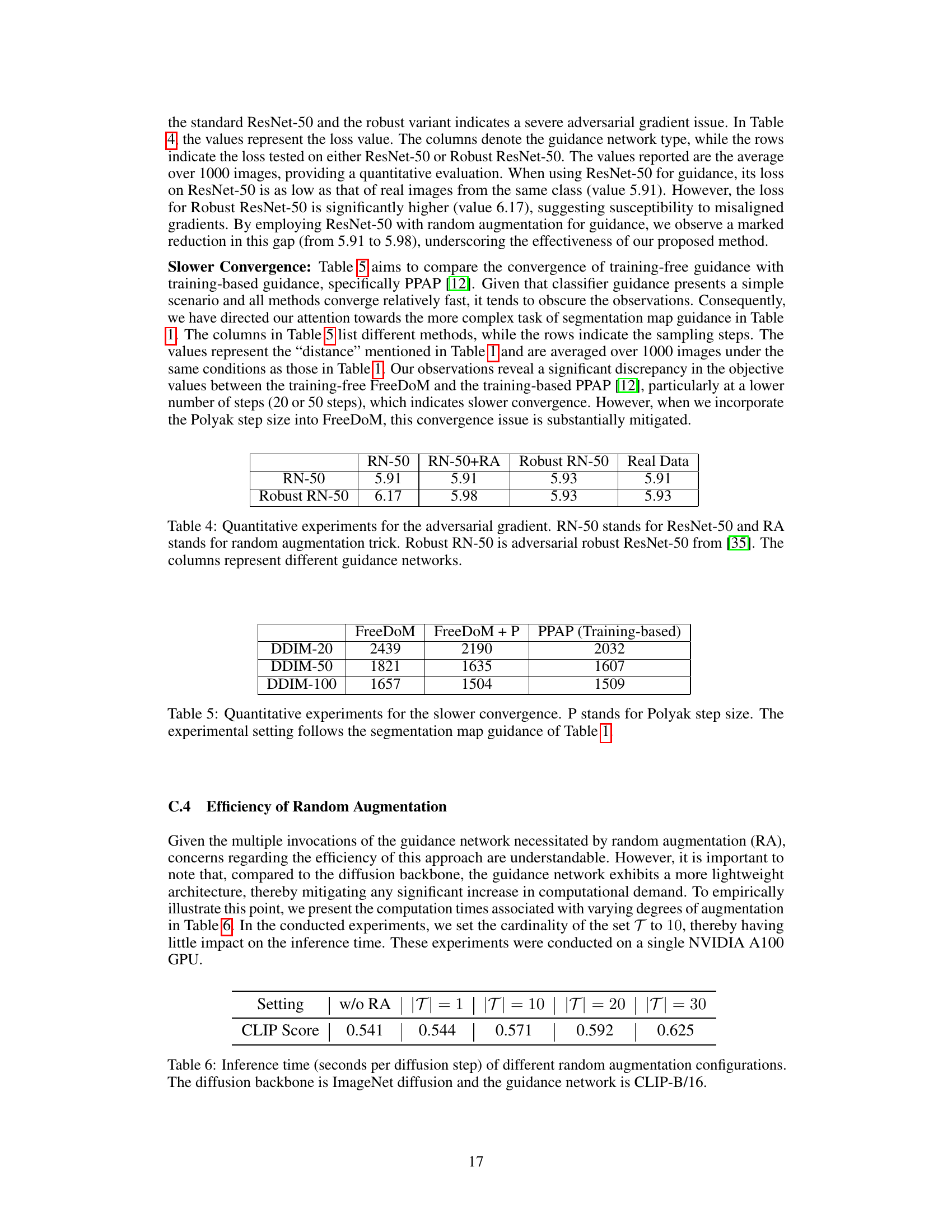
🔼 This table compares the performance of different methods on the CelebA-HQ dataset using three types of zero-shot guidance: segmentation maps, sketches, and text descriptions. The FID (Fréchet Inception Distance) and Distance metrics are used to evaluate the quality of the generated images. Lower FID and Distance scores indicate better performance. The experimental settings are consistent with those reported in another paper (reference [49]).
read the caption
Table 1: The performance comparison of various methods on CelebA-HQ with different types of zero-shot guidance. The experimental settings adhere to Table 1 of [49].

🔼 This table presents a quantitative analysis of the adversarial gradient issue in training-free guidance. It compares the loss values obtained using different guidance networks (ResNet-50, ResNet-50 with random augmentation, and a robust ResNet-50) against the loss from real images. The results demonstrate the impact of random augmentation on mitigating misaligned gradients.
read the caption
Table 4: Quantitative experiments for the adversarial gradient. RN-50 stands for ResNet-50 and RA stands for random augmentation trick. Robust RN-50 is adversarial robust ResNet-50 from [35]. The columns represent different guidance networks.

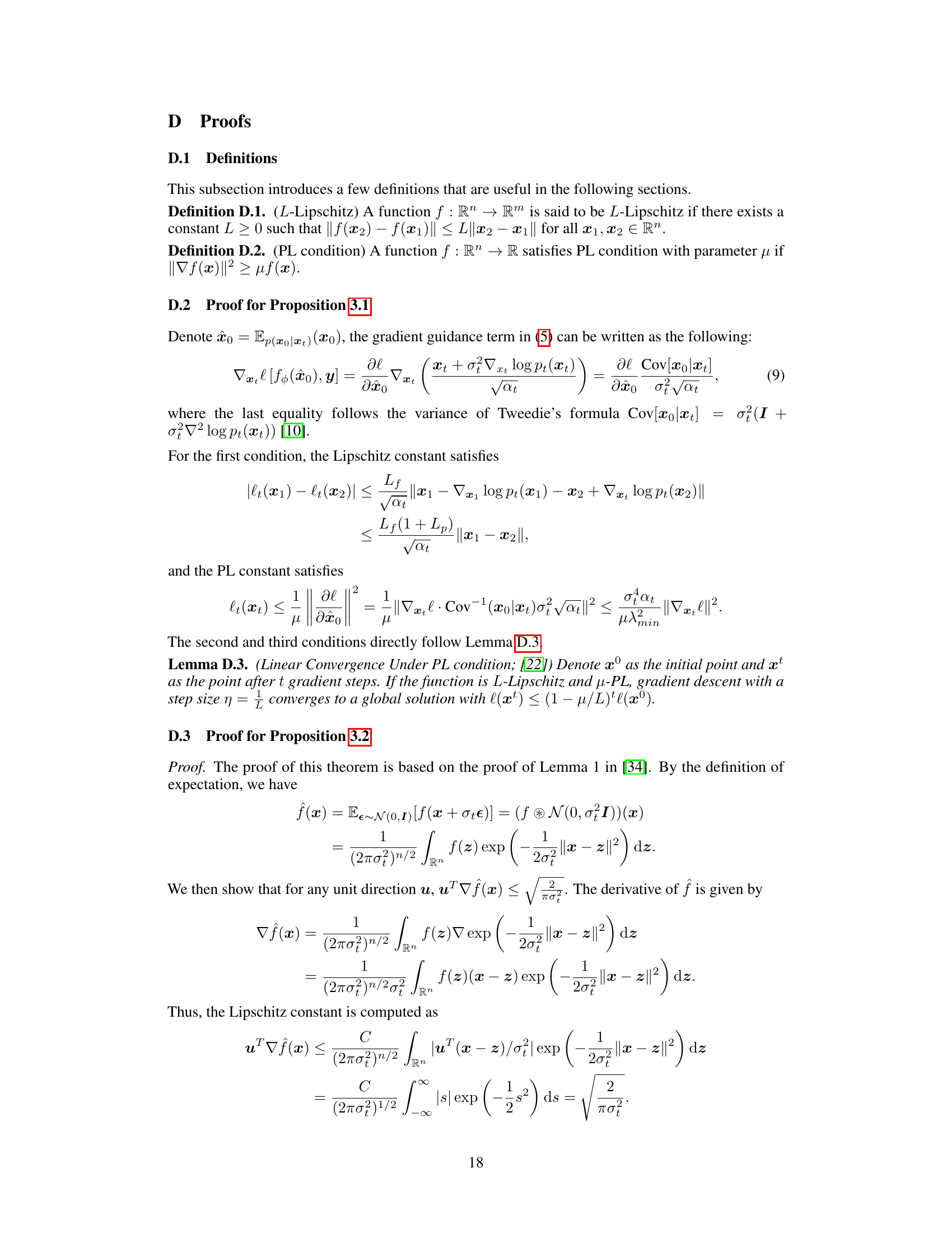
🔼 This table compares the convergence speed of training-free guidance methods (FreeDoM with and without Polyak step size) against a training-based method (PPAP) for image generation using different numbers of DDIM sampling steps (20, 50, and 100). The values represent the ‘distance’ metric from Table 1, averaged over 1000 images under the same conditions.
read the caption
Table 5: Quantitative experiments for the slower convergence. P stands for Polyak step size. The experimental setting follows the segmentation map guidance of Table 1.
Full paper#

