↗ OpenReview ↗ NeurIPS Homepage ↗ Chat
TL;DR#
Zero-shot node classification struggles with prediction bias, where unseen nodes are misclassified as seen ones. Existing methods often rely on external knowledge, neglecting the rich information within the graph structure itself. This paper introduces SpeAr, a novel method that addresses this limitation.
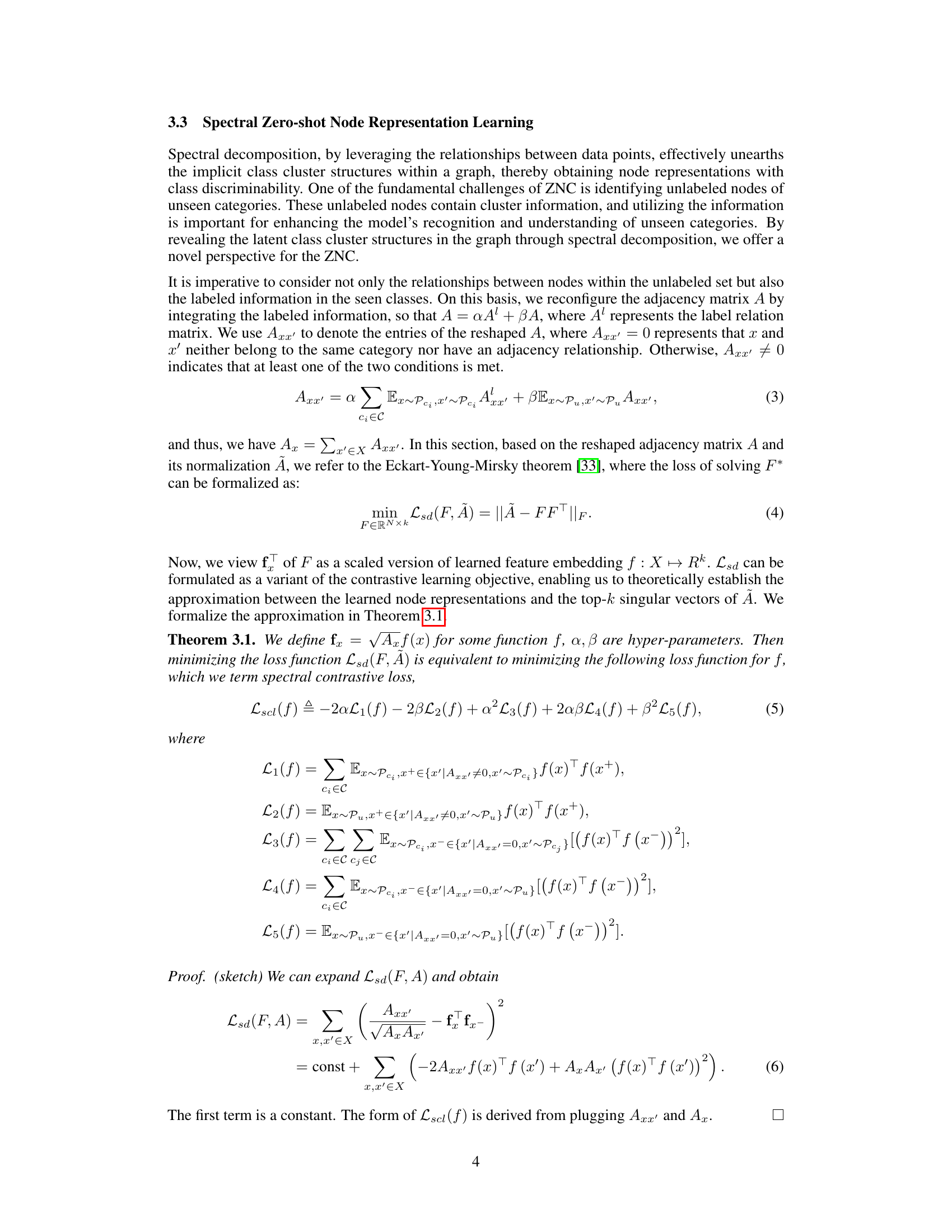
SpeAr uses spectral analysis to understand the intrinsic structure of the graph, revealing hidden class clusters. It combines this with learnable class prototypes, initialized using semantic vectors and refined iteratively. By minimizing a spectral contrastive loss, SpeAr achieves better node representation and reduces prediction bias, significantly improving performance on benchmark datasets. The two-stage training process further enhances the model’s ability to handle both seen and unseen classes, demonstrating a significant improvement over existing techniques.
Key Takeaways#
Why does it matter?#
This paper is crucial for researchers in graph data processing and zero-shot learning. It addresses the critical problem of prediction bias in zero-shot node classification by leveraging inherent graph structure. The proposed spectral approach, SpeAr, offers a novel way to effectively handle unseen classes by combining spectral analysis with learnable prototypes. This opens avenues for improved model generalization and more robust handling of dynamic graph data, areas of significant current interest.
Visual Insights#

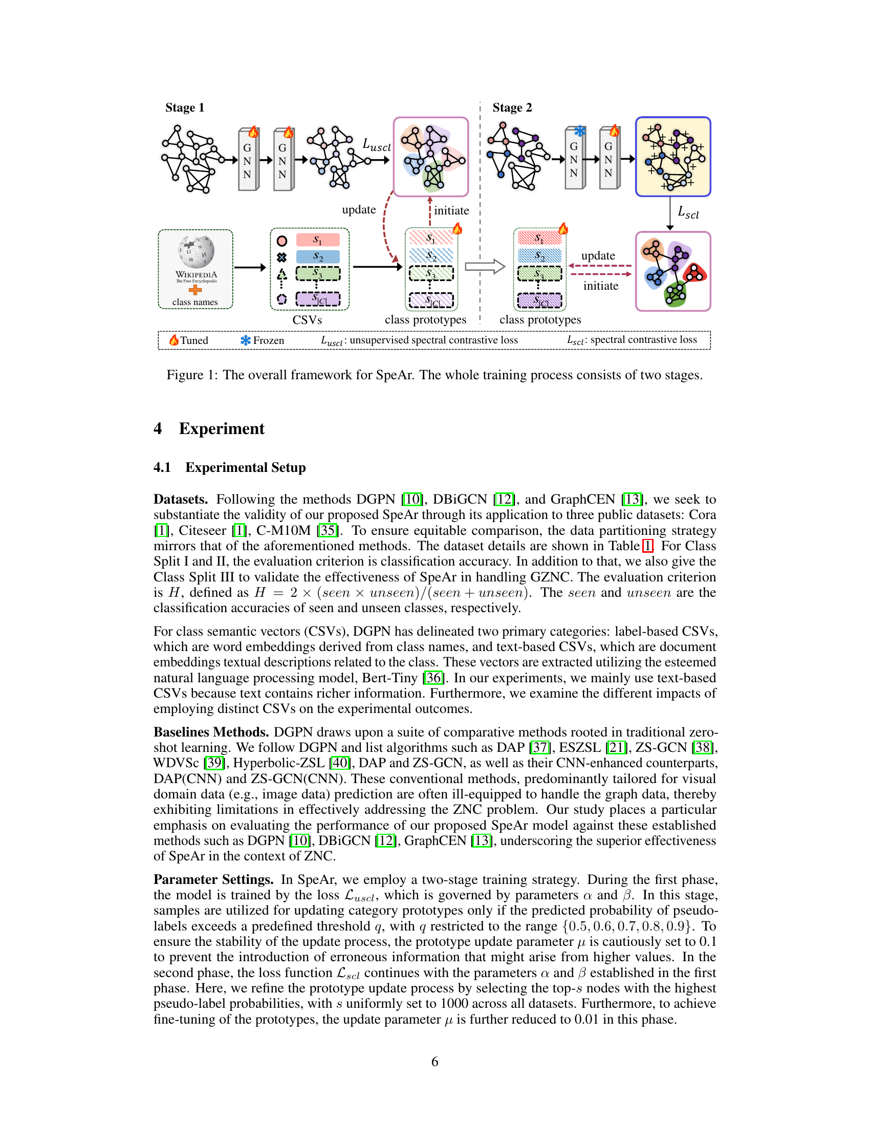
The figure illustrates the SpeAr model’s training process, which is divided into two stages. Stage 1 uses an unsupervised spectral contrastive loss (Luscl) to learn initial node embeddings and class prototypes from the graph data and class semantic vectors (CSVs). The class prototypes are initialized using CSVs. In Stage 2, a supervised spectral contrastive loss (Lscl) refines these embeddings and prototypes using both labeled and unlabeled data. This iterative process improves node representation and class separation, ultimately enhancing the model’s zero-shot node classification performance. The colored nodes indicate seen classes in the first stage and both seen and unseen classes in the second stage.

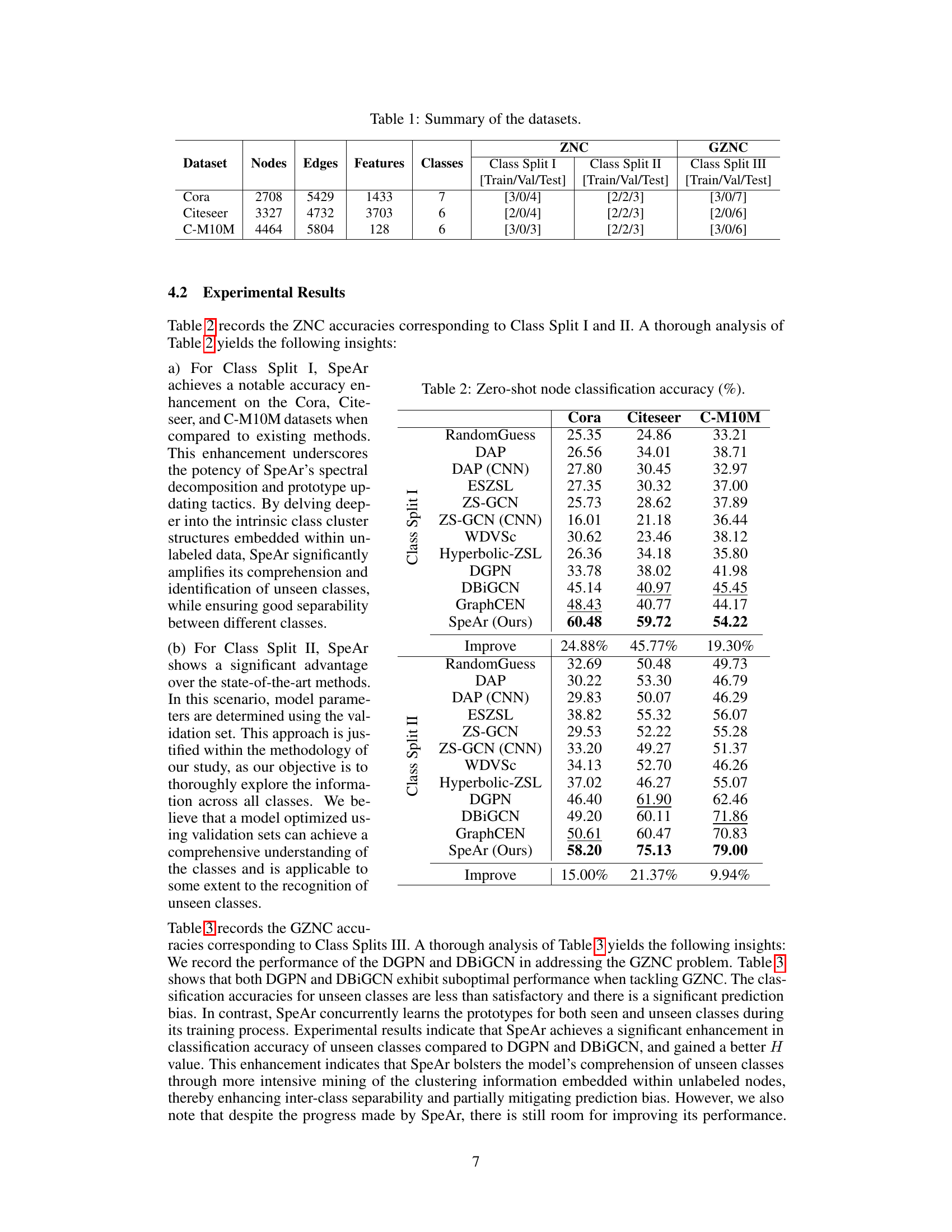
This table summarizes the characteristics of three datasets used in the experiments: Cora, Citeseer, and C-M10M. For each dataset, it provides the number of nodes, edges, features, and classes. Additionally, it shows the train/validation/test splits used for three different zero-shot node classification (ZNC) and generalized zero-shot node classification (GZNC) settings (Class Split I, II, and III). These splits define how the data is divided for training and evaluation in each experimental setting.
In-depth insights#
Spectral ZNC#
A hypothetical research paper section titled “Spectral ZNC” would likely detail a novel approach to zero-shot node classification (ZNC) leveraging spectral graph theory. The core idea would revolve around using spectral decomposition of the graph’s adjacency matrix to obtain low-dimensional node embeddings that capture inherent graph structure and cluster information. These embeddings, rich in relational context, would then be used to train a classifier capable of recognizing unseen node classes. The method might involve techniques like spectral clustering to identify latent class structures within the unlabeled nodes, potentially combined with contrastive learning to enhance the discriminative power of the embeddings. A key advantage of this approach could be its ability to effectively utilize inherent graph structure, avoiding the need for external knowledge sources (such as semantic vectors) that are often noisy and may introduce bias, while still achieving high accuracy. The section would likely include theoretical analysis demonstrating the relationship between spectral properties of the graph and class separability, as well as empirical results showcasing improved performance over existing ZNC methods. Challenges and limitations, such as computational cost for large graphs and sensitivity to noise in the graph data, would also be addressed.
Bias Mitigation#
Mitigating bias in zero-shot node classification is crucial for reliable predictions on unseen nodes. Existing methods often rely on external knowledge, such as semantic vectors, to bridge the gap between seen and unseen classes. However, this approach can be limited and may not fully capture the inherent structure of the graph. A more effective strategy focuses on leveraging the inherent cluster information within the unlabeled nodes. This approach uses spectral analysis techniques to discover implicit class structures, thus improving generalization. This is done by using techniques such as spectral contrastive loss that enables better learning of node representations and iterative refinement of class prototypes. This helps to ensure that the model is not overly reliant on biased labeled data and can effectively predict the correct labels for nodes belonging to unseen classes. Furthermore, incorporating techniques to manage the imbalance between seen and unseen data and using appropriate evaluation metrics can further enhance bias mitigation. Addressing bias requires a holistic approach that combines effective feature engineering, robust model architectures, and careful model training and evaluation. It requires an understanding of the biases present in the data, and careful consideration of how those biases impact the model’s predictions.
Prototype Learning#
Prototype learning, in the context of zero-shot node classification, is a crucial technique for effectively leveraging semantic information to classify nodes belonging to unseen classes. The core idea is to represent each class by a prototype vector, ideally capturing the essence of that class in the embedding space. Initially, these prototypes might be derived from external knowledge sources, such as pre-trained word embeddings or semantic vectors. However, the effectiveness of the prototypes significantly depends on their ability to accurately reflect the inherent cluster structure of the graph data. Therefore, iterative refinement of the prototypes is often employed, using the learned node embeddings to progressively adjust the prototypes towards better alignment with the actual class distributions. This iterative process involves updating the prototypes based on the predicted labels, often using pseudo-labels for unlabeled nodes. The performance of such a method largely relies on the choice of an effective loss function that guides the prototype learning, helping to minimize intra-class variance and maximize inter-class separation in the embedding space. Finally, the refined prototypes are utilized to classify unseen nodes by measuring the similarity (e.g., cosine similarity) between the prototype vectors and the node representations. The quality of the initial prototypes and the sophistication of the refinement mechanism are key factors determining the accuracy of zero-shot node classification.
Large-Scale ZNC#
Large-scale zero-shot node classification (ZNC) presents a significant challenge due to the computational complexity of handling massive graphs. Existing ZNC methods often struggle with scalability, as they typically involve intricate computations across the entire graph structure. A naive application of these methods to large graphs quickly becomes computationally infeasible, hindering their practical utility. Therefore, efficient algorithms and strategies are crucial for tackling large-scale ZNC. Approaches like subgraph sampling or approximation techniques may be necessary to manage the computational burden. However, these strategies could introduce biases and affect the accuracy. Developing techniques that balance computational efficiency and accuracy is vital for practical applications. Furthermore, considerations for distributed computing and parallel processing become critical for handling the immense data involved in large-scale graphs, leading to the need for robust and scalable architectures.
Future Works#
The ‘Future Works’ section of a research paper on zero-shot node classification using spectral analysis could explore several promising avenues. Extending the model to handle dynamic graphs, where nodes and edges are constantly added or removed, is crucial for real-world applicability. Investigating the impact of different graph structures on the model’s performance and exploring techniques to adapt to various graph topologies would be valuable. Improving computational efficiency is key, perhaps through exploring approximate spectral decomposition methods or more efficient optimization strategies. Furthermore, a thorough investigation into the effect of different class semantic vector representations on the model’s performance is warranted, exploring ways to leverage alternative embedding methods or incorporating additional sources of semantic information. Finally, a comparative study against state-of-the-art zero-shot learning techniques from other domains, such as image or natural language processing, would highlight the model’s strengths and weaknesses and identify areas for further improvement.
More visual insights#
More on figures
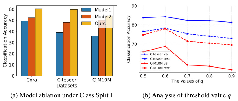
The figure illustrates the two-stage training process of the SpeAr model. Stage 1 involves unsupervised spectral contrastive loss (Luscl) to initialize class prototypes using semantic vectors (CSVs). The graph neural network (GNN) generates node embeddings. Stage 2 uses supervised spectral contrastive loss (Lscl) to refine class prototypes iteratively based on updated node embeddings, leading to improved classification accuracy. The figure shows the flow of information and the processes of initialization and update steps of the two stages. Different colors of nodes indicate different node states.

This figure shows the impact of parameters α and β on the classification accuracy across three different datasets: Cora, Citeseer, and C-M10M. Each subplot represents a dataset. The x-axis represents the value of α, and the y-axis represents the value of β. The height of each bar represents the classification accuracy achieved with the given parameter combination. The visualization helps to understand the relative contribution of labeled and unlabeled samples in the spectral contrastive loss function (Lscl).

The radar chart visualizes the performance of different zero-shot node classification models (DGPN, DBiGCN, and SpeAr) across various categories, showcasing SpeAr’s superior ability to mitigate prediction bias by achieving higher recall in multiple categories compared to other models.

This figure compares the performance of three different zero-shot node classification methods (DGPN, DBIGCN, and SpeAr) on the Citeseer dataset. Each radar chart visualizes the recall (a measure of how well the model identifies nodes belonging to a specific class) for three different classes: Artificial Intelligence, Human-Computer Interaction, and Database. The SpeAr model exhibits substantially better recall across all three classes, particularly for classes with low recall in other methods (Artificial Intelligence and Human-Computer Interaction). This demonstrates the model’s improved ability to correctly classify nodes from unseen classes and to mitigate prediction bias.
More on tables
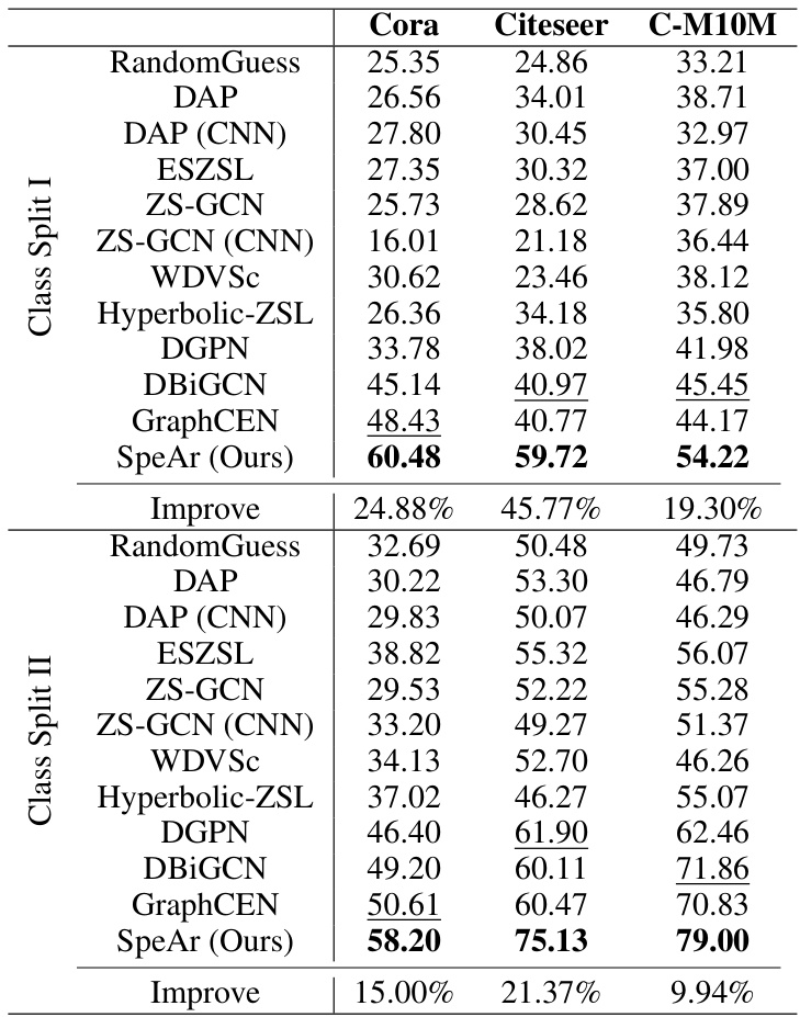
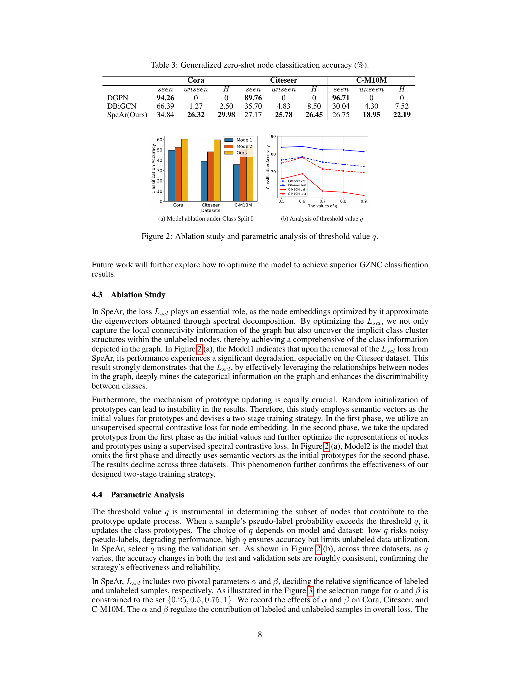
This table presents the zero-shot node classification accuracy results for different models on three benchmark datasets (Cora, Citeseer, and C-M10M). Two class split scenarios are shown: Class Split I (a small number of labeled nodes) and Class Split II (a larger number of labeled nodes). The table compares the accuracy of SpeAr (the proposed method) to several baseline methods, highlighting the improvement achieved by SpeAr in both scenarios.

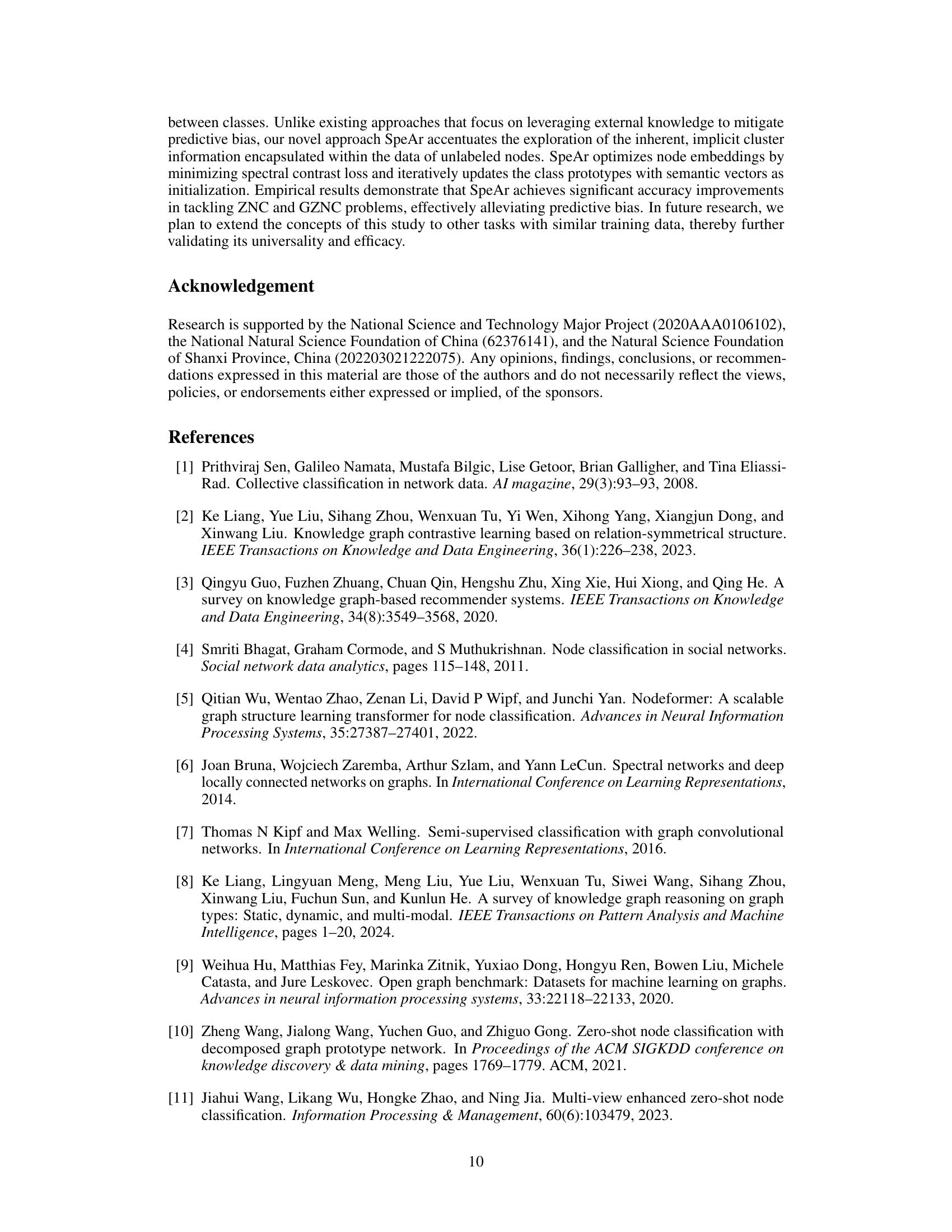
This table presents the results of generalized zero-shot node classification experiments on three datasets (Cora, Citeseer, and C-M10M). The table compares the performance of three different methods: DGPN, DBIGCN, and SpeAr (the proposed method). For each method, the table reports the classification accuracy for both seen and unseen classes, as well as the overall harmonic mean (H) of these accuracies. The harmonic mean provides a balanced measure of performance across seen and unseen classes, which is particularly important in the context of zero-shot learning where the goal is to generalize to unseen data.

This table presents the results of a comparative performance analysis between three existing zero-shot node classification methods (DGPN, DBIGCN, and GraphCEN) and the proposed SpeAr method. The comparison is performed on the large-scale Ogbn-arxiv dataset using two different data splits (Class Split I and Class Split II). The results show the classification accuracy (%) achieved by each method on both data splits. The table highlights SpeAr’s superior performance compared to the existing methods.

This table compares the performance of various zero-shot node classification models (DAP, ESZSL, ZS-GCN, WDVSc, Hyperbolic-ZSL, DGPN, DBIGCN, and SpeAr) across three datasets (Cora, Citeseer, and C-M10M) using different class semantic vectors (CSVs). It shows the classification accuracy for both TEXT-based and LABEL-based CSVs and calculates the decline rate when switching from TEXT-based to LABEL-based CSVs. The table highlights the effectiveness of SpeAr in achieving high accuracy across datasets, especially with TEXT-based CSVs. The decline rate suggests the impact of different semantic representations on model performance.
Full paper#
