TL;DR#
Many neuroscience studies use dynamical systems to model brain activity. However, accurately reconstructing these systems from real neuroimaging data (like fMRI) is difficult. Current methods often require long time series and fail when measurements depend on a history of states due to signal filtering. This is problematic because such measurements are common in neuroimaging. The paper tackles this issue.
This paper proposes a novel algorithm called convSSM to solve the problem. convSSM uses a clever method (Wiener deconvolution) to effectively train a state-space model on short, filtered neuroimaging data. The researchers demonstrate that convSSM significantly outperforms existing methods, scales efficiently to high dimensions, and accurately recovers system dynamics from short time series. They also introduce a new evaluation scheme for selecting DSR models based on short time series.
Key Takeaways#
Why does it matter?#
This paper is crucial for researchers in neuroscience and machine learning because it presents a novel, scalable method for reconstructing brain dynamics from short neuroimaging time series. It directly addresses the limitations of existing methods that struggle with data modalities exhibiting filtering properties, such as fMRI BOLD signals. The proposed convSSM algorithm offers improved accuracy and efficiency, paving the way for more sophisticated analyses of large-scale brain dynamics and personalized predictions of brain dysfunction.
Visual Insights#
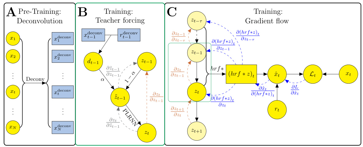
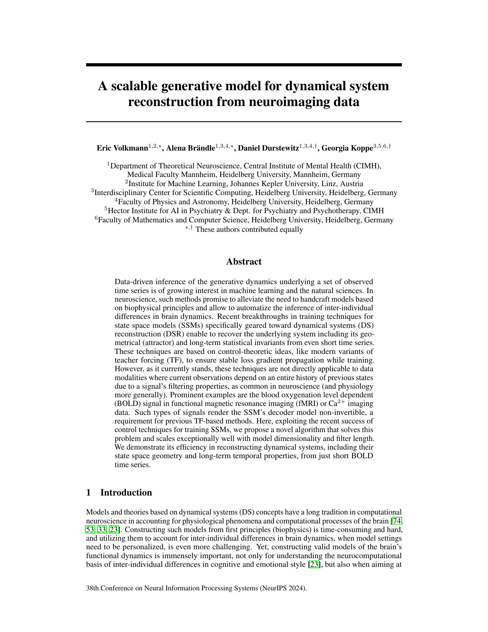
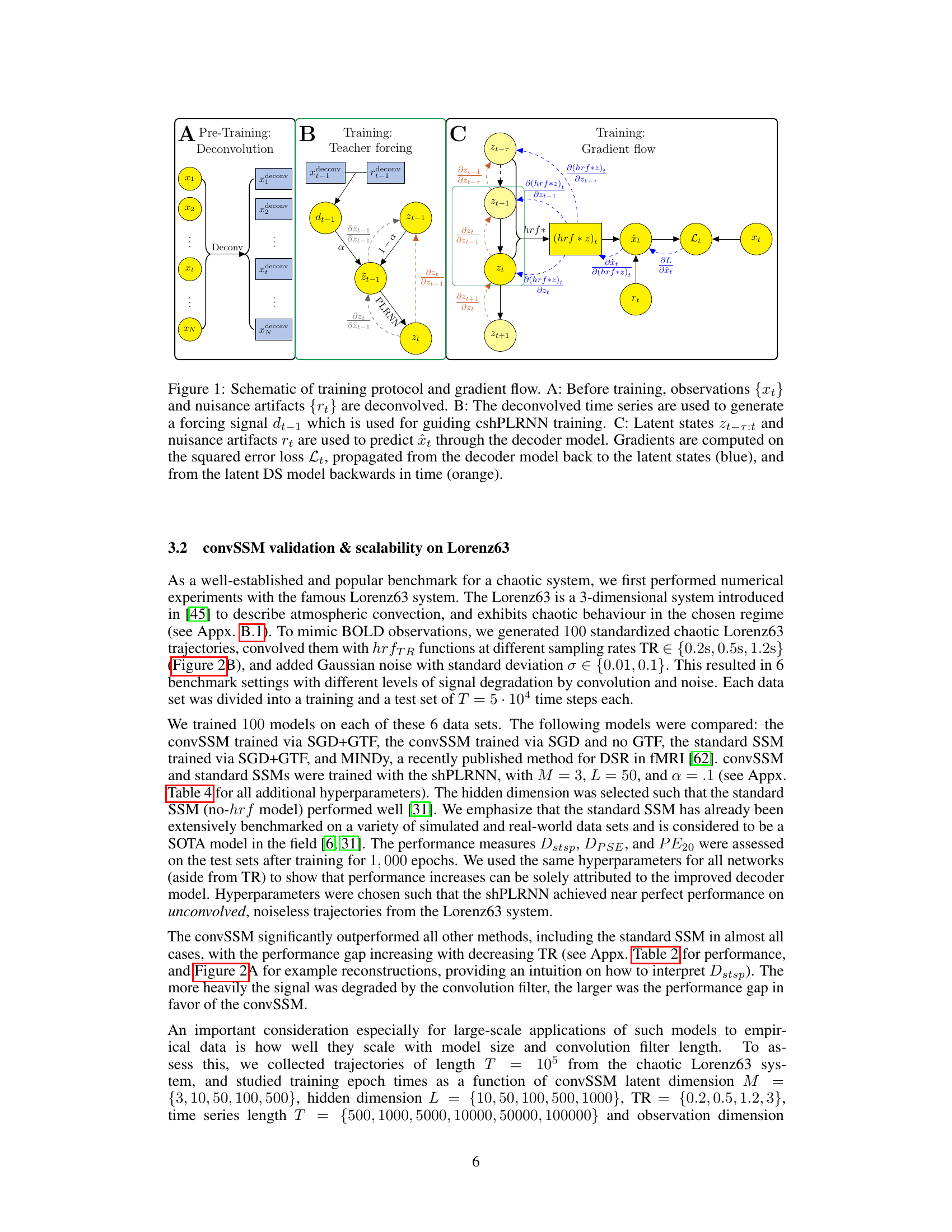
🔼 This figure illustrates the training process of the convSSM model. It shows three stages: pre-training (deconvolution of observations and artifacts), training (teacher forcing using deconvolved time series to guide cshPLRNN), and gradient flow (backpropagation from decoder to latent states and then back in time through PLRNN). The figure uses color-coded arrows to represent the flow of gradients and data.
read the caption
Figure 1: Schematic of training protocol and gradient flow. A: Before training, observations {xt} and nuisance artifacts {rt} are deconvolved. B: The deconvolved time series are used to generate a forcing signal dt-1 which is used for guiding cshPLRNN training. C: Latent states zt-r:t and nuisance artifacts rt are used to predict ît through the decoder model. Gradients are computed on the squared error loss Lt, propagated from the decoder model back to the latent states (blue), and from the latent DS model backwards in time (orange).

🔼 This table compares the performance of different dynamical systems reconstruction (DSR) models on the LEMON fMRI dataset. The metrics used are Dstsp (state space divergence, measuring geometrical overlap of orbits in state space), DPSE (power spectrum error), and 10-step PE (prediction error). The results show the convSSM generally outperforms other methods, particularly in terms of Dstsp and DPSE.
read the caption
Table 1: DSR measures evaluated for the convSSM, standard SSM, convSSM trained without GTF, as well as MINDy [62], rSLDS [44] and LFADS [14], trained on the LEMON dataset. Model runs were excluded if the 1-step PE > 1 on the training data.
In-depth insights#
ConvSSM Algorithm#
The ConvSSM algorithm, a novel approach to dynamical system reconstruction (DSR), directly addresses the limitations of previous methods when dealing with neuroimaging data. Unlike earlier techniques that assume current observations depend solely on the present latent state, ConvSSM incorporates the signal’s inherent filtering properties by utilizing a convolutional observation model. This innovation allows it to handle data modalities such as fMRI or calcium imaging where observations reflect a history of past latent states. The algorithm’s effectiveness stems from its integration of Wiener deconvolution to invert the non-invertible decoder model, enabling the use of existing efficient control-theoretic training techniques like generalized teacher forcing (GTF). Crucially, ConvSSM demonstrates excellent scalability, handling high model dimensionality and filter lengths efficiently. This scalability makes it highly suitable for real-world neuroimaging applications where data often involves high-dimensional measurements and considerable temporal dependencies. The algorithm’s success in reconstructing complex systems, including geometric properties, from relatively short BOLD time series further underscores its potential in neuroscience research.
BOLD fMRI Analysis#
BOLD fMRI analysis is a crucial technique for investigating brain activity, leveraging the blood-oxygen-level-dependent (BOLD) signal’s correlation with neuronal activity. Analyzing BOLD fMRI data involves intricate steps: preprocessing (motion correction, artifact removal, spatial smoothing), statistical analysis (general linear model, GLM), and interpretation of results to understand brain regions’ activation patterns. Challenges include low temporal resolution, indirect measurement of neuronal activity, and susceptibility to various artifacts. Advances in analysis techniques, such as independent component analysis (ICA) and dynamic causal modeling (DCM), allow researchers to move beyond simple activation maps toward understanding functional connectivity and causal relationships within brain networks. Future directions may focus on enhancing temporal resolution, incorporating multi-modal data, and developing more sophisticated analysis techniques that account for the complex neurovascular coupling process, improving the interpretation of BOLD fMRI data to reveal more nuanced insights into brain function.
DSR Model Training#
Dynamical systems reconstruction (DSR) model training presents unique challenges due to the inherent complexity of the systems being modeled. Teacher forcing (TF), a crucial technique, guides the model’s learning by feeding it ground truth states during training, which ensures stable gradient propagation and mitigates the issue of exploding gradients commonly faced when training recurrent networks on chaotic data like those encountered in neuroscience. However, standard TF methods struggle with data modalities where observations are filtered, such as fMRI BOLD signals. This paper addresses this limitation by introducing a novel approach that effectively handles convolution in the observation model via Wiener deconvolution. This allows the algorithm to still leverage the benefits of TF-based training while accurately reflecting the temporal dependencies of the signal, enabling more efficient and accurate DSR from short time series, a major advance for real-world applications where long, clean data is rarely available. The algorithm’s scalability with model dimensionality and filter length makes it particularly suitable for high-dimensional neuroimaging data. The incorporation of control-theoretic ideas and the evaluation scheme for model selection using short time series are vital contributions, enhancing the reliability and practicality of the method.
Scalability and Limits#
A crucial aspect of any machine learning model is its scalability—how well it handles larger datasets and higher-dimensional spaces. This paper investigates the scalability of its novel algorithm for dynamical systems reconstruction (DSR) by assessing performance across varying model sizes and convolution filter lengths. Results demonstrate that the algorithm scales efficiently, suggesting its suitability for applications involving extensive neuroimaging data. However, inherent limitations exist, particularly concerning the length of the time series. While the method successfully reconstructs dynamical systems from short BOLD time series, its accuracy is naturally impacted by data scarcity. The findings underscore the importance of evaluating models’ performance using metrics that capture long-term temporal and geometrical properties rather than short-term prediction errors, to ensure robustness and generalizability. Further research is needed to explore the algorithm’s behavior with even longer time series and higher-dimensional datasets, and to determine the practical limits of applicability given constraints on data availability.
Future DSR Research#
Future research in dynamical systems reconstruction (DSR) should prioritize scalability and robustness. Current methods often struggle with high-dimensional data and noisy signals, common in real-world applications like neuroimaging. Addressing this requires developing more efficient algorithms, potentially leveraging advances in sparse modeling or other dimensionality reduction techniques. Incorporating prior knowledge from domain experts (e.g., biophysical models in neuroscience) can significantly improve reconstruction accuracy and interpretability. Further exploration of causal inference within the DSR framework is needed to move beyond mere description of dynamics to understanding the underlying mechanisms driving them. Finally, benchmarking efforts should focus on creating more standardized and challenging datasets that better reflect real-world complexities, leading to more reliable comparisons of different DSR methods.
More visual insights#
More on figures

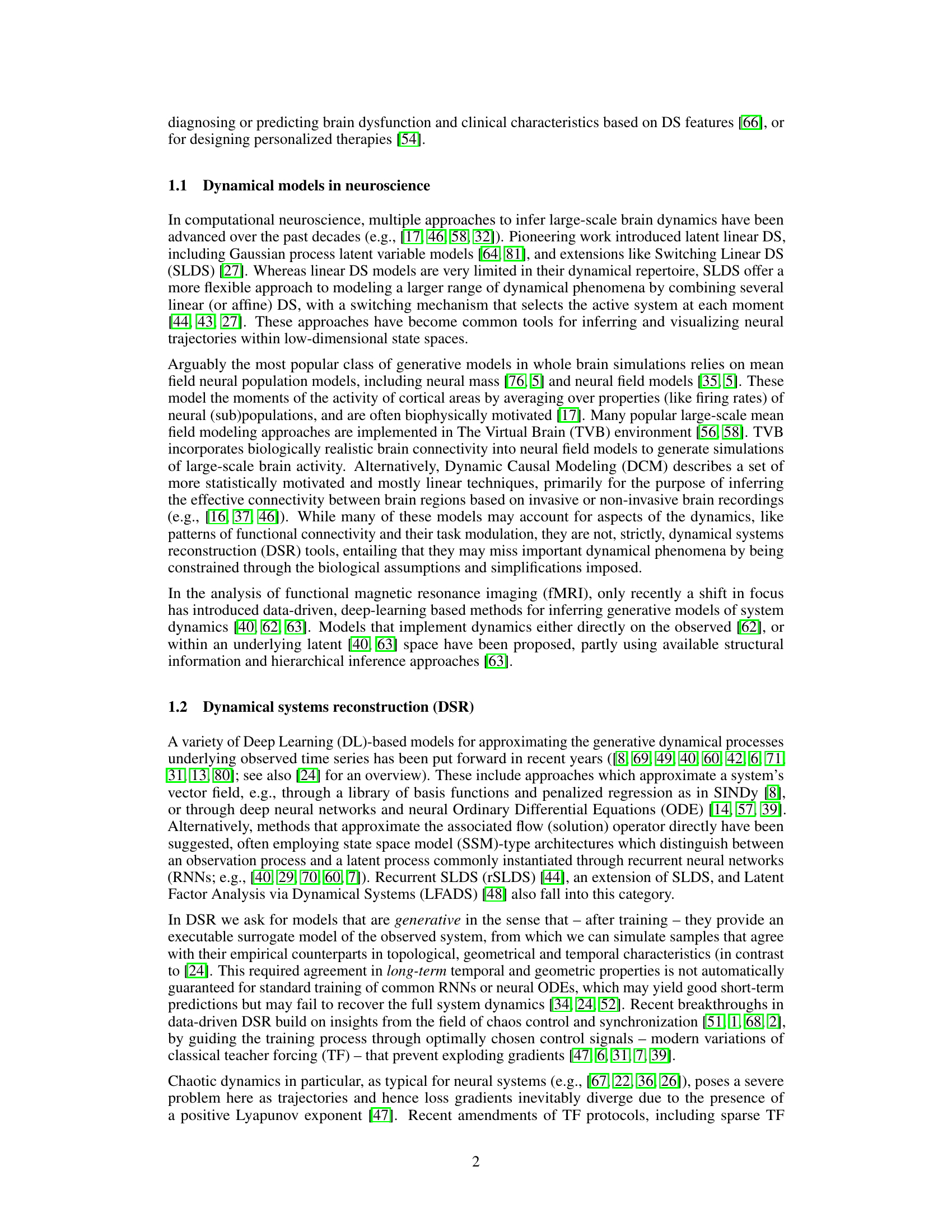
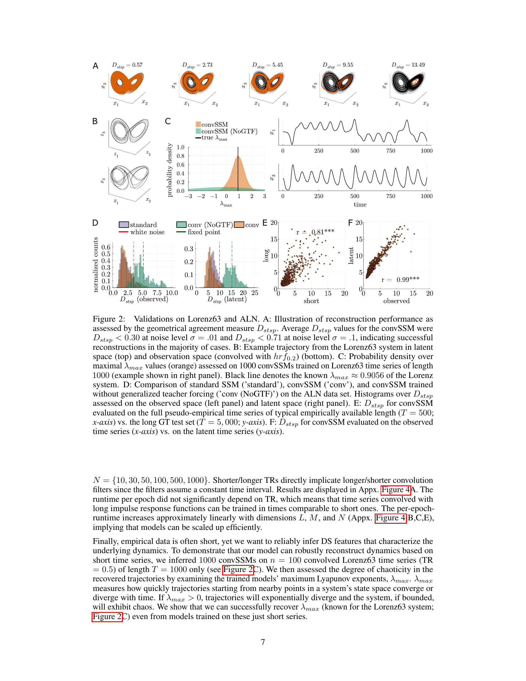
🔼 This figure shows several validations and evaluations of the convSSM model on the Lorenz63 and ALN datasets. It includes visualizations of the model’s reconstruction performance using geometrical agreement measure (Dstsp), probability density of maximal Lyapunov exponent (Amax), and histograms of Dstsp on different datasets. It also shows scatter plots comparing Dstsp values on short time series with long time series and latent space with observation space.
read the caption
Figure 2: Validations on Lorenz63 and ALN. A: Illustration of reconstruction performance as assessed by the geometrical agreement measure Dstsp. Average Dstsp values for the convSSM were Dstsp < 0.30 at noise level σ = .01 and Dstsp < 0.71 at noise level σ = .1, indicating successful reconstructions in the majority of cases. B: Example trajectory from the Lorenz63 system in latent space (top) and observation space (convolved with hrf0.2) (bottom). C: Probability density over maximal Amax values (orange) assessed on 1000 convSSMs trained on Lorenz63 time series of length 1000 (example shown in right panel). Black line denotes the known Amax ≈ 0.9056 of the Lorenz system. D: Comparison of standard SSM ('standard'), convSSM ('conv'), and convSSM trained without generalized teacher forcing ('conv (NoGTF)') on the ALN data set. Histograms over Dstsp assessed on the observed space (left panel) and latent space (right panel). E: Dstsp for convSSM evaluated on the full pseudo-empirical time series of typical empirically available length (T = 500; x-axis) vs. the long GT test set (T = 5,000; y-axis). F: Dstsp for convSSM evaluated on the observed time series (x-axis) vs. on the latent time series (y-axis).
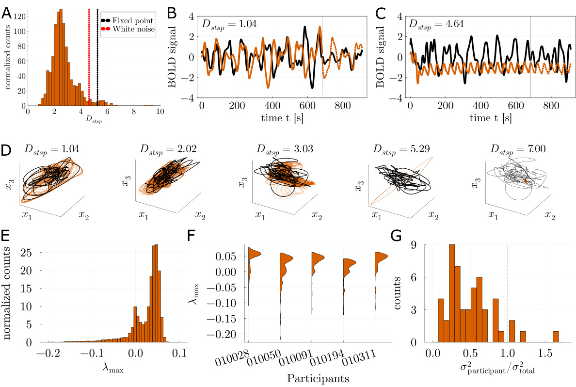
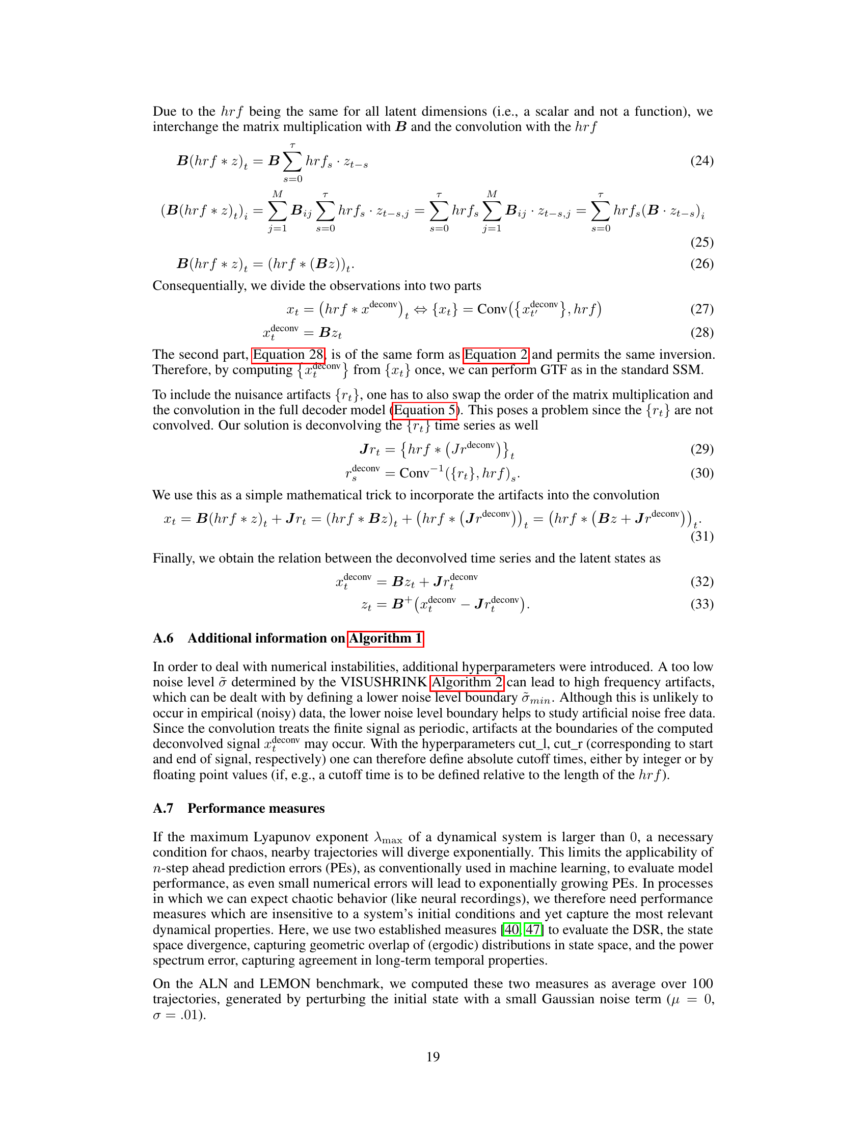
🔼 This figure demonstrates the model’s performance on the Lorenz63 and ALN datasets. It shows that the convSSM model accurately reconstructs the dynamics of these systems, even with noisy or convolved data. Key performance metrics such as Dstsp and DPSE are compared across different models and conditions. The figure highlights the convSSM’s superior performance and scalability, especially when dealing with short time series.
read the caption
Figure 2: Validations on Lorenz63 and ALN. A: Illustration of reconstruction performance as assessed by the geometrical agreement measure Dstsp. Average Dstsp values for the convSSM were Dstsp < 0.30 at noise level σ = .01 and Dstsp < 0.71 at noise level σ = .1, indicating successful reconstructions in the majority of cases. B: Example trajectory from the Lorenz63 system in latent space (top) and observation space (convolved with hrf0.2) (bottom). C: Probability density over maximal Amax values (orange) assessed on 1000 convSSMs trained on Lorenz63 time series of length 1000 (example shown in right panel). Black line denotes the known Amax ≈ 0.9056 of the Lorenz system. D: Comparison of standard SSM ('standard'), convSSM ('conv'), and convSSM trained without generalized teacher forcing ('conv (NoGTF)') on the ALN data set. Histograms over Dstsp assessed on the observed space (left panel) and latent space (right panel). E: Dstsp for convSSM evaluated on the full pseudo-empirical time series of typical empirically available length (T = 500; x-axis) vs. the long GT test set (T = 5,000; y-axis). F: Dstsp for convSSM evaluated on the observed time series (x-axis) vs. on the latent time series (y-axis).
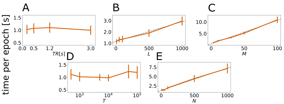
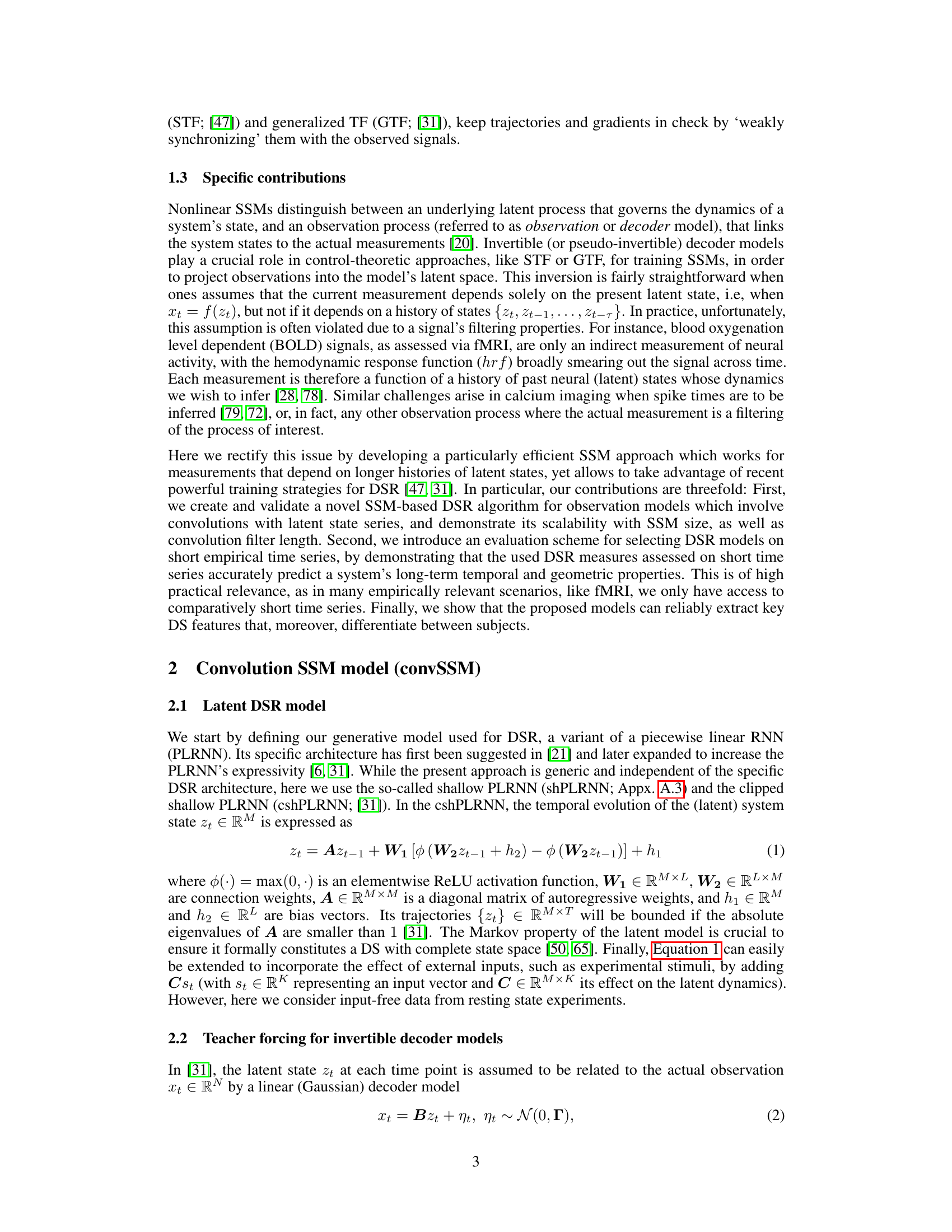
🔼 This figure shows the scalability of the convSSM model. The training time per epoch is plotted against different model parameters (TR, L, M, T, N). The results demonstrate that the training time increases approximately linearly with the model dimensionality and filter length, indicating good scalability.
read the caption
Figure 4: Training duration per epoch (y-axis) in seconds for different TRs (A), hidden dimensions L (B), latent dimensions M (C), time series length (D), and observation dimensions (E). Mean, standard error (SEM) and linear curve fits (gray dashed lines) are displayed. The per-epoch-runtime increases approximately linearly with dimensions L, M, and N; explained variance R² = 0.989, R₁ = 0.993, and R = 0.996 for linear regressions with predictors 'L', 'M', and 'N', respectively. Experiments were performed on a standard notebook with Intel i5-8250U 1,60 GHz CPU and 8GB RAM.
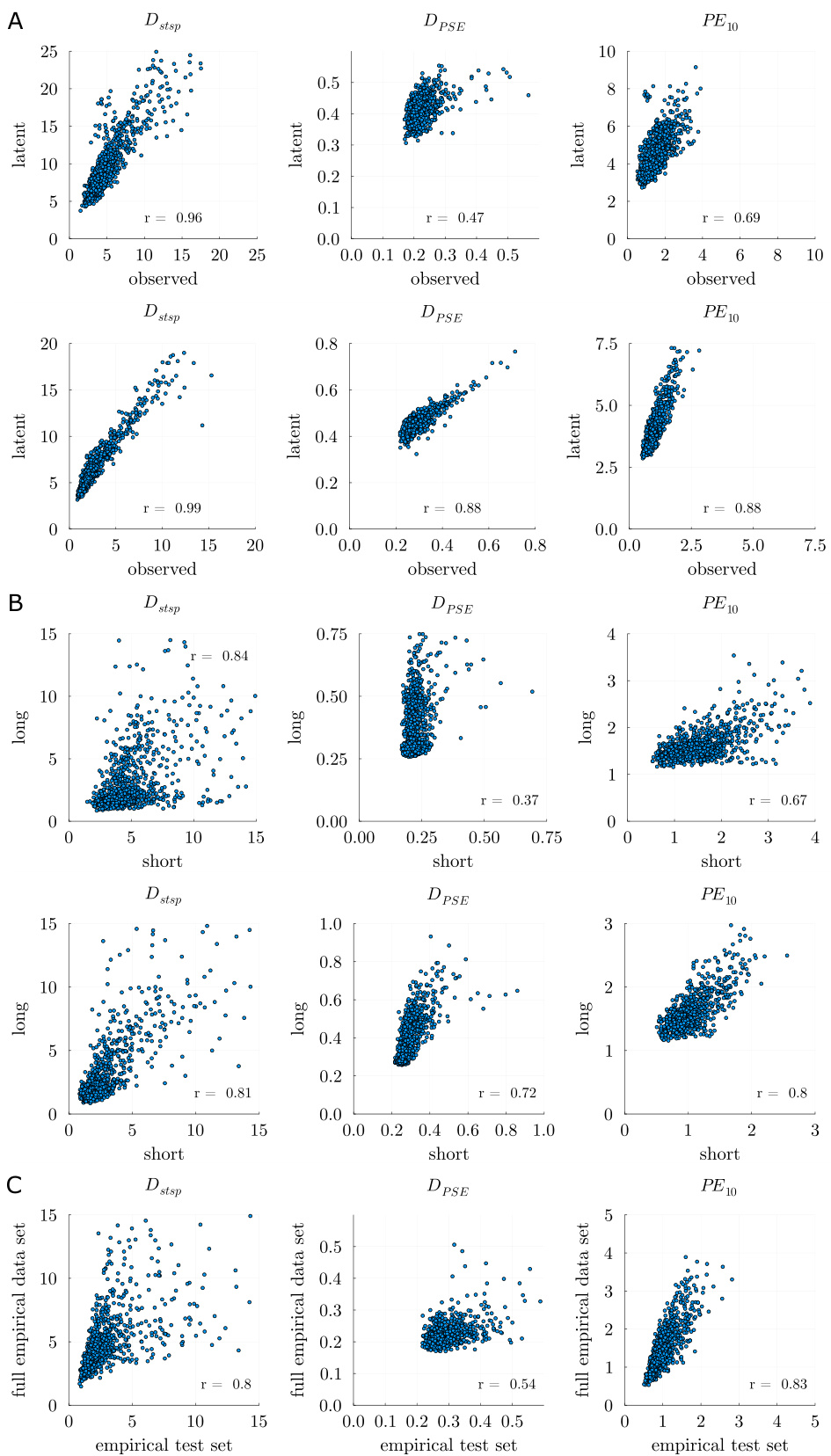
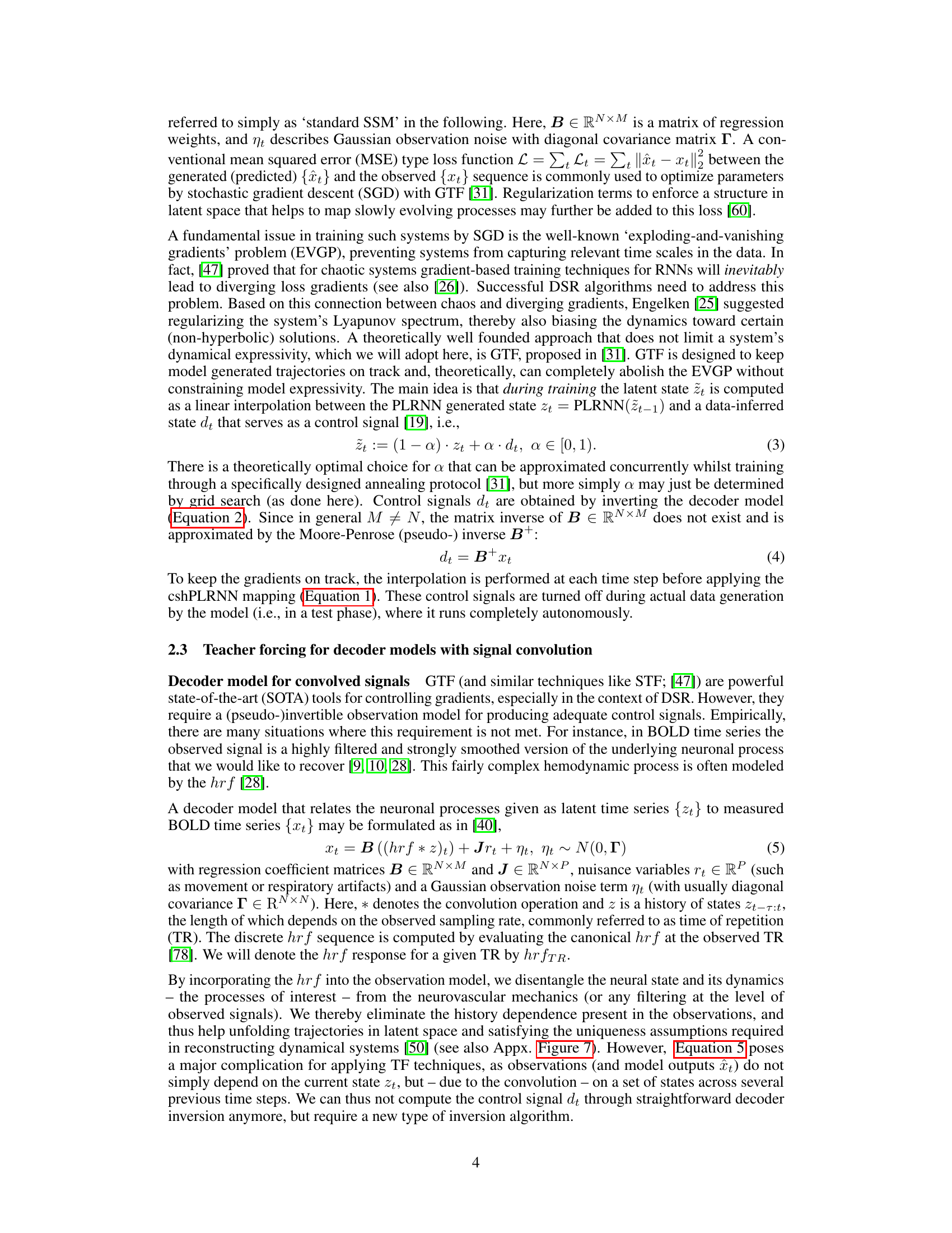
🔼 This figure demonstrates the agreement between the different DSR measures (Dstsp, DPSE, and PE10) when evaluated on different subsets of the ALN dataset. Panel A shows the agreement between measures calculated on the short pseudo-empirical test set and the full pseudo-empirical time series. Panel B displays the correlation between the same measures using short pseudo-empirical time series and longer time series (GT test set). Panel C shows the agreement between measures on the pseudo-empirical test set and the full pseudo-empirical time series.
read the caption
Figure 5: A: Agreement in DSR measures assessed on the observed (x-axis) vs. latent (y-axis) space of the short pseudo-empirical test set (top) and the full pseudo-empirical time series (bottom). Correlations between Dstsp (left), DPSE (middle), and PE10 (right) are displayed, respectively. B: Top: Agreement in DSR measures assessed on the pseudo-empirical test set (short) vs. GT test set (long). Bottom: Same for full pseudo-empirical time series (short) vs. GT test set (long). Correlations between Dstsp (left), DPSE (middle), and PE10 (right) are displayed, respectively. C: Correlations between DSR measures between pseudo-empirical test set and full pseudo-empirical time series, same order as in B.
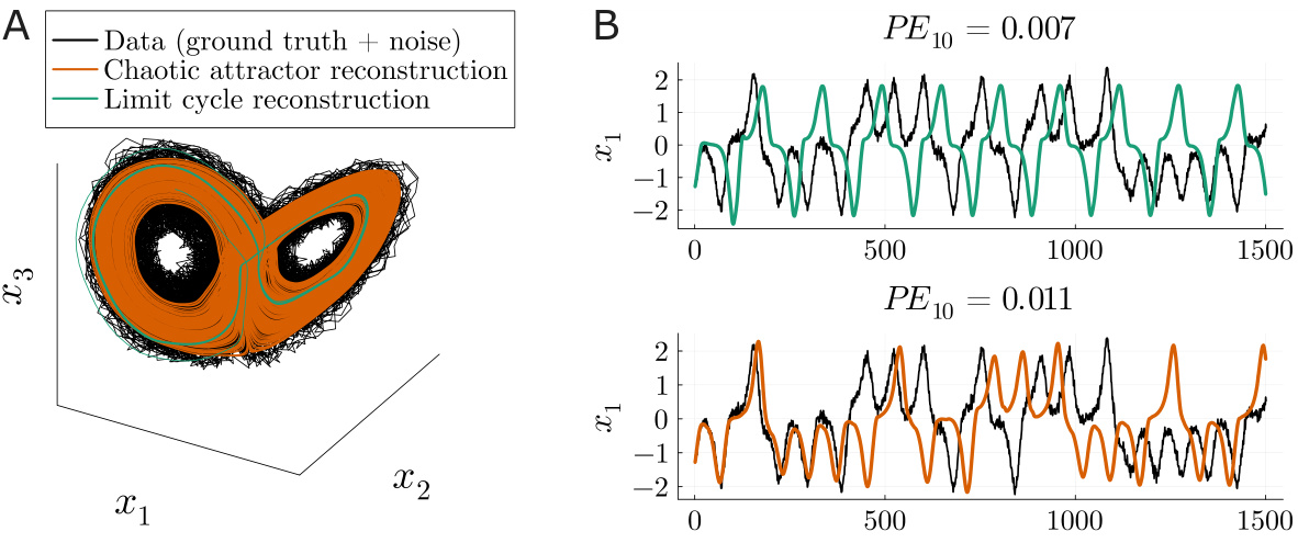
🔼 This figure shows a comparison between a good and a bad reconstruction of a Lorenz attractor. The ground truth data (black) is shown along with a good reconstruction (orange) and a bad reconstruction (green). The good reconstruction accurately captures the shape of the attractor, while the bad reconstruction produces a limit cycle instead of a chaotic attractor. The bottom panel plots the corresponding time series for each of the reconstructions and the ground truth. The figure highlights the fact that simple prediction error (PE) is not a suitable metric to evaluate the quality of dynamical system reconstruction, as the inaccurate model achieves a lower PE than the accurate one.
read the caption
Figure 6: A. Ground truth Lorenz trajectory sampled with noise (black), a good reconstruction with low Dstsp (orange) that accurately recovers the attractor, and a poor reconstruction with high Dstsp (green) that represents the attractor inaccurately, yielding an oscillatory (limit cycle) instead of a chaotic solution. B. Trajectories of systems in A. unfolded in time. The inaccurate reconstruction (top) achieves a lower prediction error (PE) than the accurate reconstruction (bottom), due to trajectory divergence in chaotic systems. This example illustrates that PEs are inadequate to capture the reconstruction of chaotic DS.

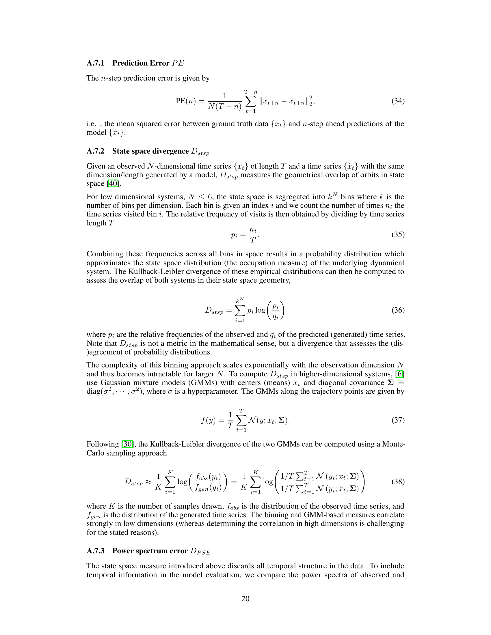
🔼 This figure demonstrates the effectiveness of the proposed deconvolution method by comparing the autocorrelation and mutual information of the latent and observed time series, both with and without removing the linear dependencies between consecutive time points. It shows that the deconvolution effectively removes the temporal dependencies in the latent states, while the dependencies remain in the observed time series. The comparison of the residual time series using both latent states and cshPLRNN model output shows that the temporal dependencies are removed effectively by the proposed deconvolution and modeling method.
read the caption
Figure 7: A: Full (solid) and residual (dashed) average (across dimensions) auto-correlation functions for the latent (left) and observed (right) time series. For the residual auto-correlation, the immediately preceding time step was regressed out. For the dotted curve, cshPLRNN(≈t−1) instead of zt−1 was regressed out. B: Same as A for the mutual information as a function of time lag.
More on tables

🔼 This table presents a quantitative comparison of the performance of standard SSM and convSSM models on the Lorenz63 dataset with added noise. Different levels of noise (σ) and convolution filter lengths (hrf) were used. The metrics reported include the mean squared prediction error (PE20), state space divergence (Dstsp), and power spectrum error (DPSE). The number of converged models (Nconverged) is also shown, indicating the proportion of successful training runs for each condition.
read the caption
Table 2: Quantitative comparison between standard SSM and convSSM on noisy Lorenz63 data (Nconverged is the number of converged models).

🔼 This table presents the results of Dynamical Systems Reconstruction (DSR) performance evaluation using three different models (convSSM, standard SSM, and convSSM without GTF) on the ALN dataset. It compares performance metrics (Dstsp, DPSE, and 10-step PE) across three different test conditions: full pseudo-empirical time series, pseudo-empirical test set, and ground truth test set, evaluating the models both in latent space and the noisy observation space of the data.
read the caption
Table 3: DSR measures evaluated on the ALN data set for the convSSM, the standard SSM, and the convSSM trained without generalized teacher forcing by setting α = 0. Measures were evaluated on the ground truth latent space and the noisy observation space on the different created test sets.
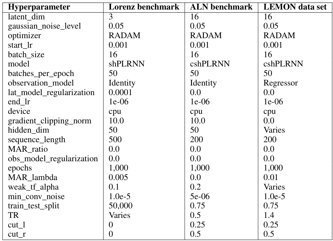
🔼 This table shows the hyperparameters used in the experiments described in the paper. It breaks down the settings used for three different benchmarks: the Lorenz63 system, the ALN model, and the LEMON dataset. For each benchmark, it shows the values used for various parameters such as the latent dimension, Gaussian noise level, optimizer used, learning rate, batch size, model type, and other relevant training parameters. Note that some parameters are given fixed values, while others vary across experiments.
read the caption
Table 4: Hyperparameter settings for the experiments conducted. 'Varies' means the respective hyperparameter was varied in the experiment.
Full paper#
