↗ OpenReview ↗ NeurIPS Homepage ↗ Chat
TL;DR#
Current dynamic scene rendering often suffers from issues like over-smoothness in implicit methods and excessive feature overlap in low-rank plane-based explicit methods, resulting in suboptimal rendering quality. These limitations hinder the creation of high-fidelity dynamic scenes, especially those with complex deformations.
Grid4D tackles these issues by employing a novel 4D decomposed hash encoding, breaking from the low-rank assumption. This, combined with a directional attention module and smooth regularization, significantly improves rendering quality and speed. The method’s effectiveness is demonstrated by experiments that show superior results compared to state-of-the-art models across various datasets.
Key Takeaways#
Why does it matter?#
This paper is important because it addresses limitations of existing dynamic scene rendering methods by proposing a novel approach that significantly improves rendering quality and speed. Its focus on high-fidelity and efficiency makes it highly relevant to current research trends in computer graphics and related fields. The research also opens new avenues for exploring improved explicit representation methods in various applications, impacting future developments in dynamic scene rendering.
Visual Insights#

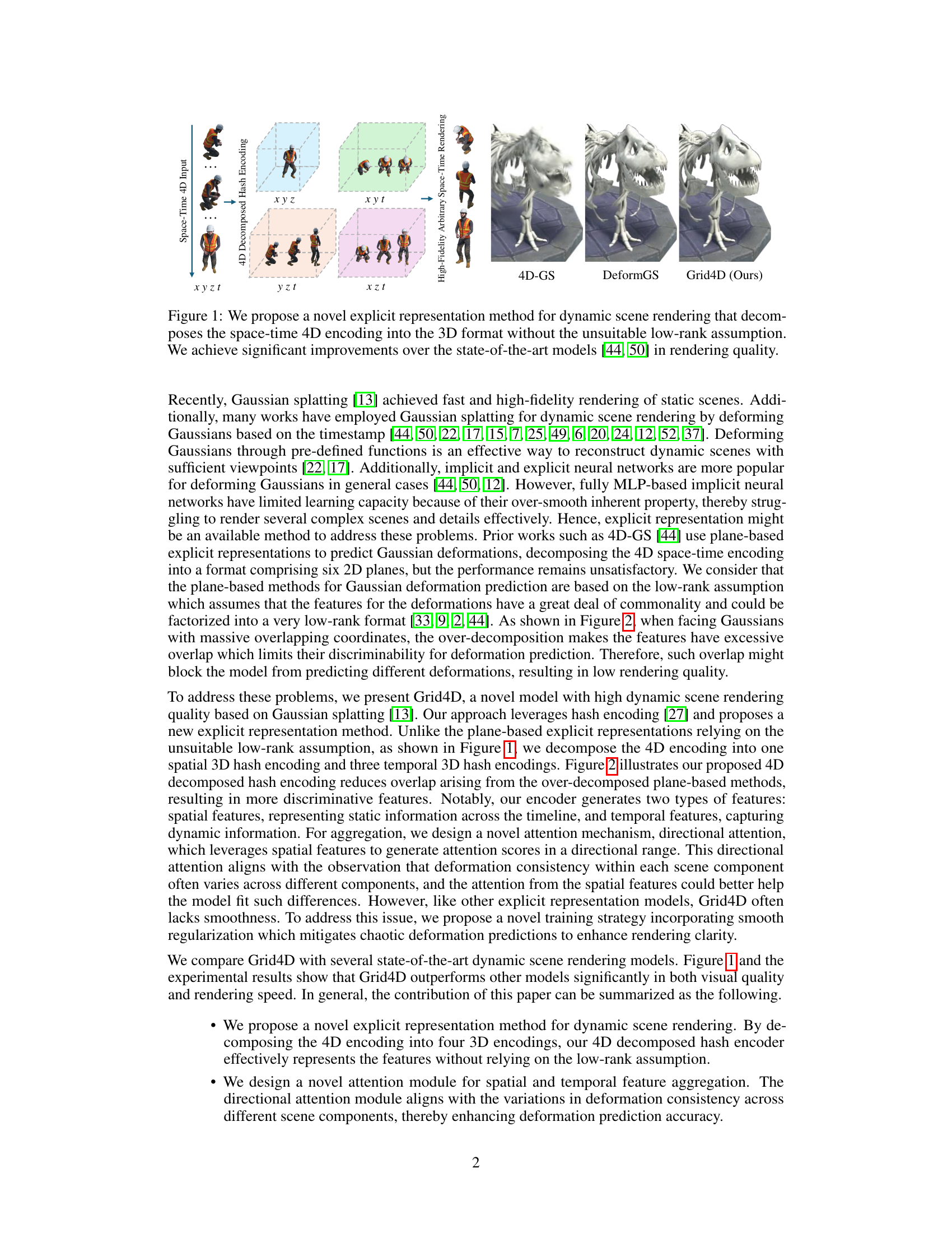
This figure shows a comparison of different dynamic scene rendering methods. The input is a 4D space-time representation of a scene. Grid4D (the proposed method) decomposes this 4D input into four 3D representations (xyz, xyt, yzt, xzt), using hash encoding, to avoid the limitations of previous plane-based methods that rely on the low-rank assumption. The figure visually demonstrates the improvement in rendering quality achieved by Grid4D compared to 4D-GS and DeformGS, showcasing more detail and better visual fidelity.
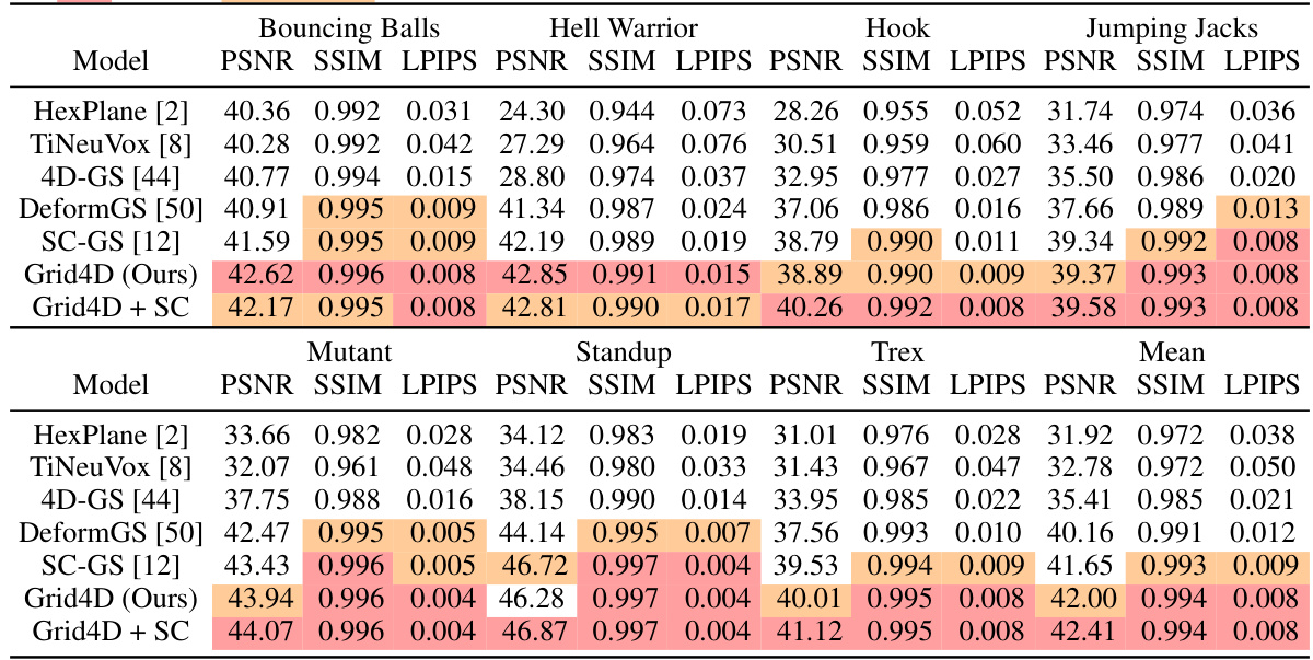
This table presents a quantitative comparison of the proposed Grid4D model against several state-of-the-art methods on the synthetic D-NeRF dataset. The metrics used for evaluation are PSNR (Peak Signal-to-Noise Ratio), SSIM (Structural Similarity Index), and LPIPS (Learned Perceptual Image Patch Similarity). Higher PSNR and SSIM values, along with lower LPIPS values, indicate better rendering quality. The table highlights the best and second-best performing methods for each scene.
In-depth insights#
4D Hash Encoding#
The concept of “4D Hash Encoding” for dynamic scene rendering presents a novel approach to efficiently represent and process spatiotemporal data. Traditional methods often rely on low-rank assumptions or excessively decompose the 4D space-time information, leading to feature overlap and reduced rendering quality. 4D Hash Encoding addresses this by decomposing the 4D input into multiple lower-dimensional (e.g., 3D) hash encodings. This decomposition strategy allows for a more discriminative feature representation, reducing overlap and enhancing the model’s ability to accurately fit diverse deformations across different scene components. The effectiveness of this approach hinges on the careful design of the hash functions and the subsequent aggregation of the lower-dimensional features. A key advantage lies in its ability to avoid the limitations of plane-based methods, which are often based on unsuitable low-rank assumptions. Furthermore, the use of hash encoding inherently offers advantages in terms of memory efficiency and rendering speed compared to fully implicit representations. Therefore, “4D Hash Encoding” shows promise in improving the quality and efficiency of dynamic scene reconstruction models.
Directional Attention#
The proposed directional attention mechanism is a key innovation designed to enhance the accuracy of deformation prediction in dynamic scene rendering. Unlike standard attention which assigns weights based solely on feature similarity, this method leverages spatial features to generate attention scores within a directional range (-1, 1). This directional aspect is crucial because deformation consistency isn’t uniform across all scene components; some areas might exhibit opposite motions. By incorporating this directional information, the model can better fit diverse deformations in complex scenes. The use of a spatial MLP to generate these scores ensures the attention weights are informed by the scene’s static structure, thereby improving the accuracy of temporal feature aggregation. This approach is a significant improvement over traditional methods that rely on low-rank assumptions or uniform attention, resulting in a more robust and detailed rendering of dynamic scenes.
Smooth Regularization#
The concept of ‘Smooth Regularization’ in the context of dynamic scene rendering, as described in the provided research paper excerpt, addresses a critical challenge posed by explicit representation methods. These methods, while offering speed advantages, often lack inherent smoothness, leading to chaotic or unnatural-looking deformations. The smooth regularization term, likely added to the loss function during training, directly penalizes large differences in predicted deformations between nearby spatial and temporal points. This effectively encourages the model to generate smoother, more continuous changes in the scene over time and space. By mitigating chaotic deformations, the approach improves the visual quality of the rendered dynamic scenes. The implementation details of this technique, such as the specific form of the regularization term and the choice of hyperparameters, are crucial for optimal performance. The success of smooth regularization highlights the trade-off between speed and accuracy in dynamic scene rendering, suggesting that carefully balancing explicit and implicit elements is key to achieving high-fidelity results.
Limitations of Grid4D#
Grid4D, while demonstrating significant advancements in high-fidelity dynamic scene rendering, exhibits certain limitations. Training speed does not see improvements compared to existing methods, possibly due to the computational overhead of the smooth regularization and the increased number of Gaussians needed for accurate deformation predictions. The method’s performance might degrade when dealing with extremely complex scenes or scenes with substantial motions, resulting in rendering artifacts, likely stemming from the challenges of the explicit representation approach, especially in handling intricate spatial-temporal relationships. While achieving real-time rendering speed for many sequences, memory consumption is a factor which is also affected by the number of Gaussians, and future work may improve this further. Furthermore, the model’s reliance on the 4D decomposed hash encoding, while innovative, might limit its ability to capture certain fine-grained details when facing heavily overlapping coordinate features. Finally, the impact of the smooth regularization on training and generalization requires additional exploration to optimize its use and potential trade-offs with rendering quality.
Future Enhancements#
Future enhancements for this research could explore several promising avenues. Improving the handling of complex motions and highly dynamic scenes remains a key challenge; the current model struggles with certain complex deformations. Investigating more sophisticated deformation models, perhaps incorporating physics-based simulations or learning more robust representations of motion, could significantly enhance performance. Addressing the training speed limitations is another important area. While the model provides high-quality results, reducing training time is crucial for wider adoption. This could involve exploring more efficient architectures, optimization techniques, or data augmentation strategies. Finally, extending the model to handle more complex scene geometries and novel view synthesis tasks would broaden its applicability. This could entail incorporating more advanced scene representations or developing new techniques for effectively handling occlusions and varying lighting conditions. Further research might also focus on developing effective methods for user interaction and control over scene dynamics.
More visual insights#
More on figures

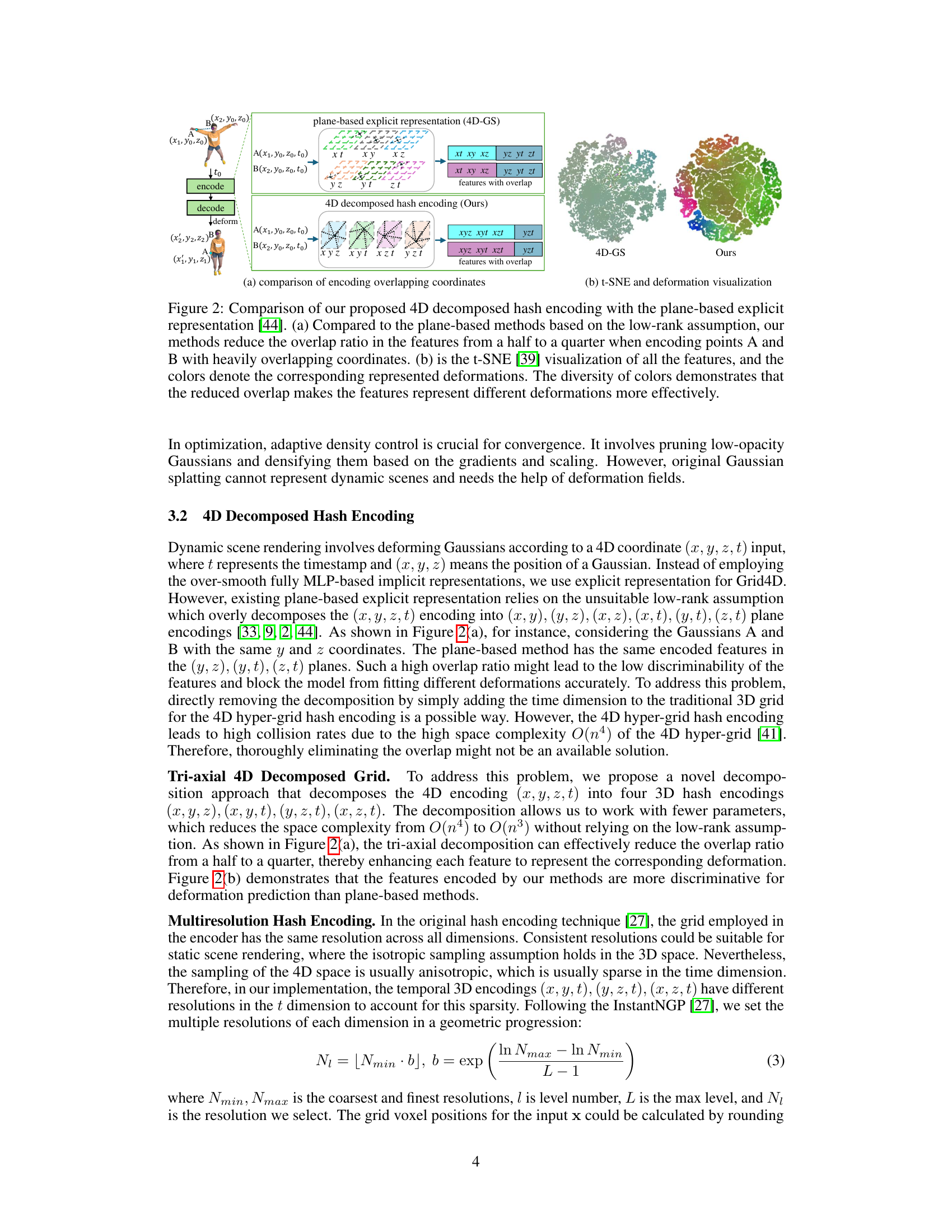
This figure compares the proposed 4D decomposed hash encoding method with the existing plane-based explicit representation method. Subfigure (a) shows how the proposed method reduces feature overlap, improving the discriminative power of the features for deformation prediction. Subfigure (b) uses t-SNE visualization to show that the reduced overlap results in features that better represent different deformations.
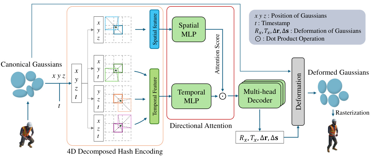
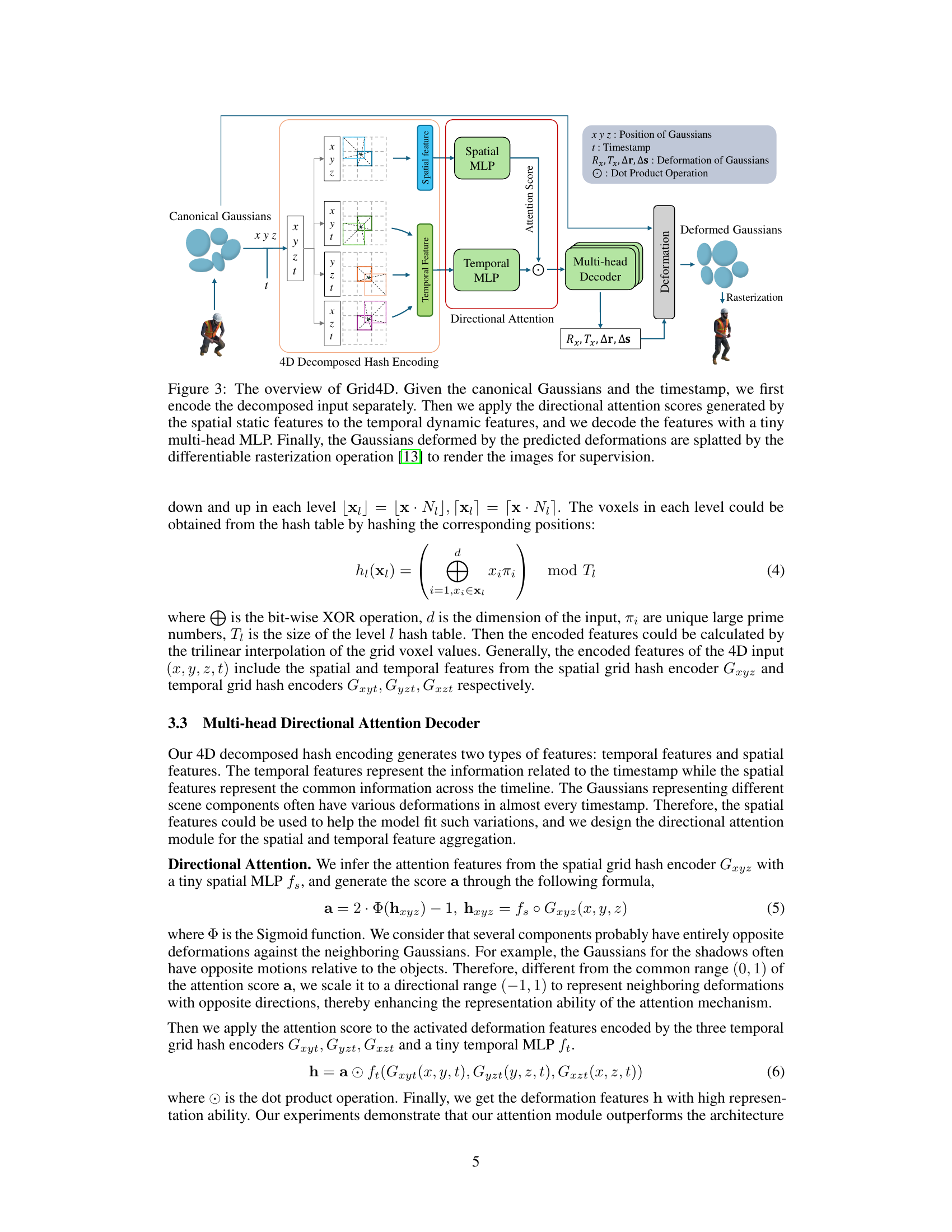
This figure shows the overall architecture of the Grid4D model. It starts with canonical Gaussians and their timestamps as input. These inputs are then processed through a 4D decomposed hash encoding, separating the spatial and temporal features. Spatial features are passed through a spatial MLP to generate directional attention scores, which are then applied to the temporal features (processed by a temporal MLP). A multi-head decoder combines these features to produce deformation parameters for the Gaussians. Finally, differentiable rasterization renders the deformed Gaussians to produce the final output images.
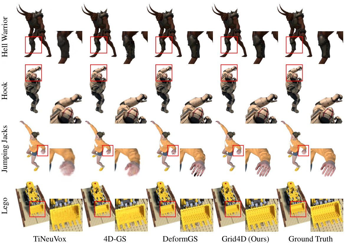
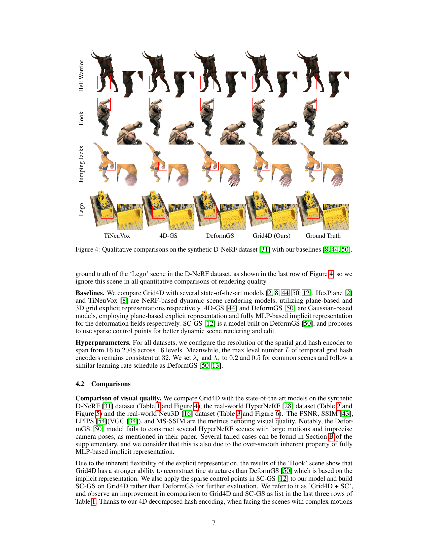
This figure compares the visual quality of scene reconstruction by Grid4D against three other state-of-the-art methods: TiNeuVox, 4D-GS, and DeformGS. Each row represents a different dynamic scene from the D-NeRF dataset, showing several frames from the sequence. The red boxes highlight areas where the differences in reconstruction quality between the methods are most apparent. The aim is to visually demonstrate that Grid4D produces higher-fidelity reconstructions compared to the baselines. Ground truth images are provided for reference.

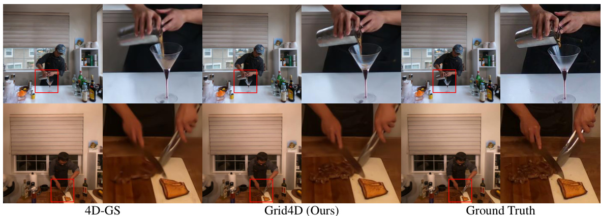
This figure compares the visual quality of several dynamic scene rendering methods on the real-world HyperNeRF dataset. The models compared are TiNeuVox, 4D-GS, DeformGS, and Grid4D (the authors’ proposed method). Each row represents a different scene with multiple frames showing the reconstruction quality at various time points. Red boxes highlight areas where differences in reconstruction are apparent. The Ground Truth row provides the original images for reference, allowing for a direct comparison of each method’s accuracy in reconstructing the dynamic scenes.
This figure compares the visual results of Grid4D with three baseline methods (4D-GS, DeformGS, TiNeuVox) on four dynamic scenes from the D-NeRF dataset. Each scene shows a sequence of frames, illustrating the model’s ability to render novel views of the dynamic scene over time. The red boxes highlight areas with fine details, showing differences in rendering quality between the models. Grid4D demonstrates superior performance in terms of visual fidelity compared to baselines, showing more detailed and accurate results that are closer to the ground truth.

This figure illustrates the overall architecture of the Grid4D model. It begins with canonical Gaussians and their timestamp as input. These inputs are then encoded separately using the 4D decomposed hash encoding method into spatial and temporal features. A directional attention mechanism combines these features, and a multi-head decoder predicts the Gaussian deformations. Finally, differentiable rasterization renders the deformed Gaussians into images, which are used for model supervision during training.

This figure shows the architecture of the multi-head directional attention decoder used in Grid4D. It illustrates the process of generating attention scores from spatial features using a small spatial MLP (Multilayer Perceptron), scaling those scores to a directional range (-1, 1), and then applying those scores to temporal features via a dot product operation before decoding the final deformation parameters using another MLP. The output of this decoder provides the deformation parameters (rotation, translation, scaling) for the Gaussians.

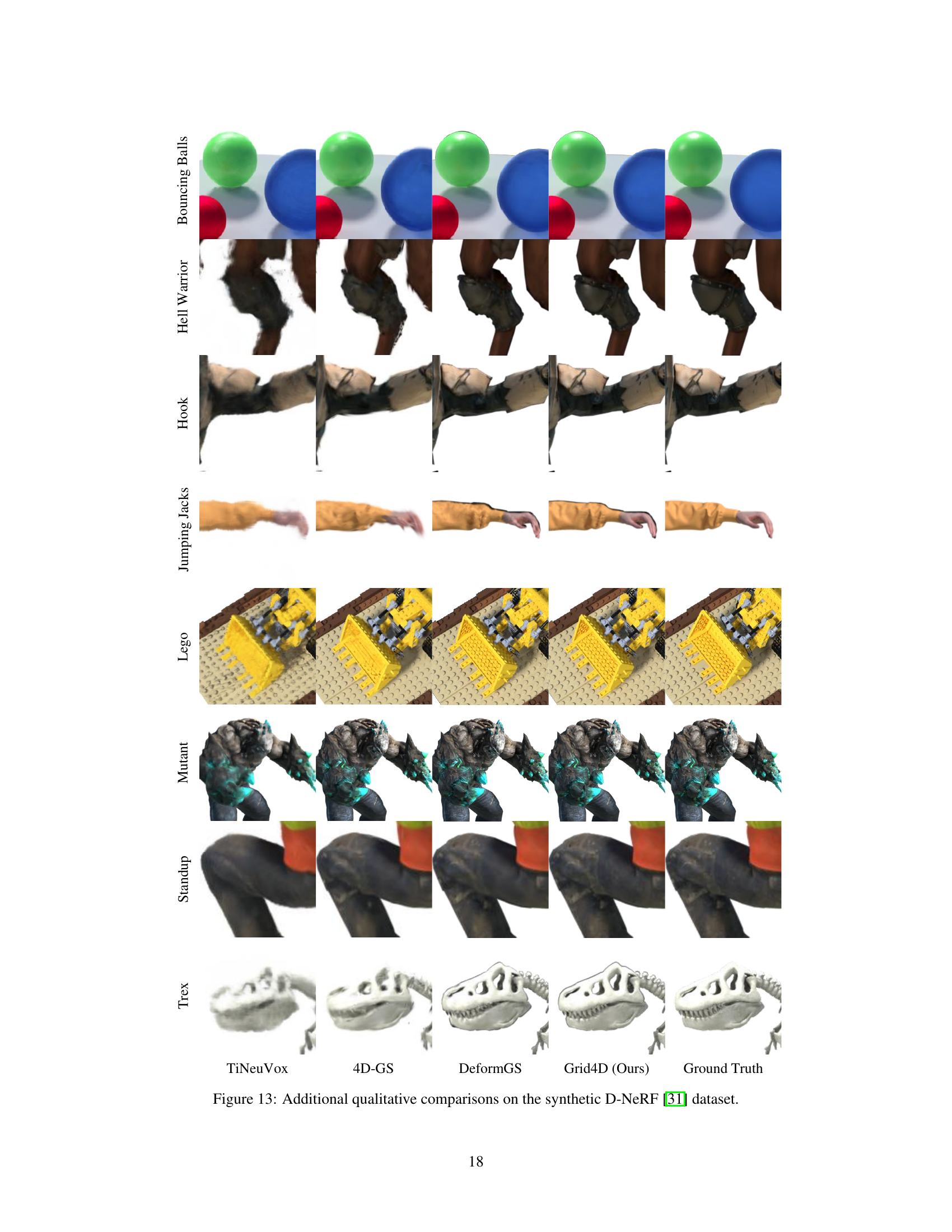
This figure shows a qualitative comparison of the dynamic scene rendering results produced by Grid4D and three baseline methods (4D-GS, DeformGS, and TiNeuVox) on four sequences from the D-NeRF dataset. Each sequence contains several frames showing different poses of the same object. The image demonstrates that Grid4D outperforms the baseline models in terms of visual quality, especially in handling complex deformations and details.

This figure shows qualitative comparisons of different dynamic scene rendering methods (TiNeuVox, 4D-GS, DeformGS, and Grid4D) on the real-world HyperNeRF dataset. Each row represents a different scene, and each column represents a different method. The ground truth images are shown in the last column. The figure visually demonstrates the performance of each method on various scenes with complex motions and dynamic objects.

This figure compares the results of three different methods for dynamic scene rendering: Space-Time 4D Input, 4D-GS, and Grid4D (the authors’ method). Each method is shown rendering the same dynamic scene from several different viewpoints. Grid4D uses a novel 4D decomposed hash encoding to represent the scene, while the other methods rely on less effective approaches. The figure demonstrates that Grid4D produces significantly higher-fidelity results.

This figure compares the visual quality of dynamic scene rendering results generated by Grid4D and three baseline methods (TiNeuVox, 4D-GS, DeformGS) on four sequences from the D-NeRF dataset. Each sequence shows a different dynamic scene (Lego, Jumping Jacks, Hook, Hell Warrior) with multiple frames representing different stages of the action. The comparison demonstrates Grid4D’s superior ability to render detailed, realistic, and sharp images compared to the baseline models, which suffer from various artifacts such as blurry edges and lack of fine details. The ground truth images are also included for reference.

This figure compares the visual quality of dynamic scene rendering results generated by Grid4D and three baseline methods (TiNeuVox [8], 4D-GS [44], DeformGS [50]) on the D-NeRF dataset. Each row represents a different dynamic scene, showing the results from the four methods and the corresponding ground truth. The comparison visually demonstrates Grid4D’s superior performance in rendering quality compared to the other methods.
More on tables

This table presents a quantitative comparison of the proposed Grid4D model against two baseline models, TiNeuVox and 4D-GS, on the HyperNeRF dataset. The evaluation metrics used are PSNR and MS-SSIM, which measure peak signal-to-noise ratio and multi-scale structural similarity index, respectively. The dataset is split into two parts: ‘Rig’ (4 scenes) and ‘Interpolation’ (6 scenes). Higher scores for PSNR and MS-SSIM indicate better rendering quality. The table highlights the best and second-best performance for each metric and scene category.

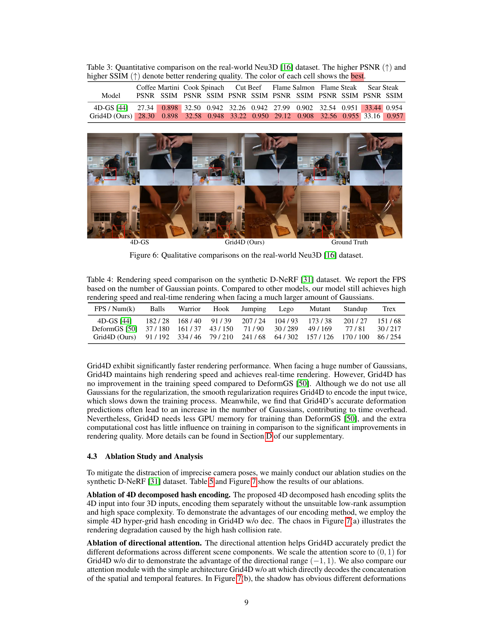
This table presents a quantitative comparison of the Grid4D model and the 4D-GS model on the Neu3D dataset. The evaluation metrics used are PSNR and SSIM, which measure peak signal-to-noise ratio and structural similarity, respectively. Higher values for both metrics indicate better visual quality. The table is organized to show the results for each scene in the dataset (Coffee Martini, Cook Spinach, Cut Beef, Flame Salmon, Flame Steak, Sear Steak). The best performing model for each metric in each scene is highlighted by color.

This table compares the rendering speed (FPS) of Grid4D against other state-of-the-art models on the synthetic D-NeRF dataset. The number of Gaussian points used in each model is also provided to allow for a fairer comparison, as different models use different numbers of Gaussians. Grid4D demonstrates high rendering speed, maintaining real-time performance even with a large number of Gaussians.

This table presents a quantitative comparison of the visual quality of different models on the HyperNeRF dataset, broken down into two parts: the validation rig and the interpolation. The metrics used are PSNR and MS-SSIM, both higher values indicate better quality. The table highlights the best and second-best performing models for each scene.

This table presents ablation study results on the model architecture, specifically focusing on the impact of different configurations of the 4D decomposed hash encoder. It compares the performance using various depths and levels within the encoder, as well as a variant without rotation and translation (w/o RT). The PSNR metric is used to evaluate the rendering quality.

This table compares the training computational cost of four different dynamic scene rendering models: 4D-GS, DeformGS, SC-GS, and Grid4D. The comparison includes training time, GPU memory usage, and the resulting PSNR (Peak Signal-to-Noise Ratio) value. Grid4D demonstrates a balance between training time and memory consumption compared to other models, while achieving a high PSNR.
Full paper#
