↗ arXiv ↗ Hugging Face ↗ Hugging Face ↗ Chat
TL;DR#
Inferring Markov jump processes (MJPs) from noisy data is notoriously difficult, requiring complex models and extensive training. Current methods often struggle with sparse or noisy observations, and their parameters are highly dataset-specific, limiting generalizability. This hinders efficient analysis of diverse dynamic systems across various scientific fields.
This research introduces a novel methodology for zero-shot inference of MJPs, addressing these limitations. Using a pretrained neural recognition model and a synthetic training dataset covering a wide range of MJPs and noise levels, the researchers successfully infer hidden MJPs from various real-world datasets with zero-shot learning. The model matches or even surpasses state-of-the-art performance on these datasets, demonstrating its effectiveness and broad applicability.
Key Takeaways#
Why does it matter?#
This paper is crucial because it presents a novel zero-shot inference methodology for Markov jump processes. This addresses a long-standing challenge in various scientific fields, enabling researchers to efficiently analyze complex dynamic systems without extensive model retraining. The work is significant due to its potential for broad applicability and its performance comparable to state-of-the-art models. It opens doors for further research into zero-shot learning and its application across numerous domains.
Visual Insights#

🔼 This figure shows two examples of dynamic processes that can be modeled using Markov jump processes (MJPs). The left panel shows a discrete flashing ratchet process, a simple model of a Brownian motor. The right panel shows current recordings from a viral potassium channel. The key takeaway is that even though these systems are very different, after a coarse graining step, their dynamics can be described by similar MJPs. This is a motivation for the authors’ work to infer MJPs from various kinds of data.
read the caption
Figure 1: Processes of very different nature (seem to) feature similar jump processes. Left: State values (blue circles) recorded from the discrete flashing ratchet process (black line). Right: Current signal (blue line) recorded from the viral potassium channel KcvMT35, together with one possible coarse-grained representation (black line).

🔼 This table presents the inference results for the discrete flashing ratchet (DFR) process. It compares the inferred parameters (V, r, b) from the ground truth, the NeuralMJP model, and the proposed Foundation Inference Model (FIM). The FIM results are averages over 15 batches, each using a context number of c(300, 50), which represents the number of data points used in the inference.
read the caption
Table 1: Inference of the discrete flashing ratchet process. The FIM results correspond to FIM evaluations with context number c(300, 50), averaged over 15 batches.
In-depth insights#
Zero-Shot MJP Inference#
The concept of ‘Zero-Shot MJP Inference’ presents a significant advancement in Markov Jump Process (MJP) modeling. Traditionally, MJP inference necessitates training a model on a specific dataset, limiting its applicability to unseen data. Zero-shot learning bypasses this limitation, enabling the model to infer hidden MJPs from diverse datasets without prior training. This is achieved by pre-training the model on a synthetic dataset encompassing a broad range of MJPs and noise characteristics, effectively creating a foundation model. The trained model generalizes well, exhibiting zero-shot inference capabilities across various datasets, including those with different state space dimensionalities. This approach significantly reduces the need for extensive dataset-specific training, proving efficient and effective for numerous real-world applications. A key advantage is the performance comparability with state-of-the-art models specifically trained on target datasets, highlighting the efficacy and generalizability of the zero-shot approach. However, limitations exist in the generalizability to data distributions significantly differing from those used during pre-training. Further refinement of the synthetic data generation model could enhance its robustness to even more diverse data.
FIM Architecture#
The Foundation Inference Model (FIM) architecture for Markov Jump Process (MJP) inference is a supervised learning approach that leverages synthetic data for training. It comprises two main components: a synthetic data generation model which simulates a broad range of MJPs with varying complexities, noise levels, and observation schemes, creating a training dataset. The second component is a neural recognition model, which processes simulated MJP observations and predicts the rate matrix and initial state distribution of the underlying MJP. This recognition model employs a combination of sequential processing (e.g., LSTM or Transformers) and attention mechanisms to capture temporal dynamics and relationships within the data. Zero-shot inference capability is a key feature, where the trained model can predict MJP parameters without requiring dataset-specific fine-tuning, showcasing the efficacy of learning from a rich, synthetic dataset that captures the essential features of the MJP space.
Synthetic Data Gen#
The heading ‘Synthetic Data Generation’ suggests a crucial methodology for training and evaluating machine learning models, specifically within the context of Markov Jump Processes (MJPs). A core challenge in MJP inference is the scarcity of real-world, accurately labeled datasets. Synthetic data generation offers a solution by creating artificial datasets that mimic the properties of real-world MJPs. This allows researchers to train and validate their models on a large quantity of data, even if real data is limited or expensive to collect. The quality of the synthetic data is paramount. A well-designed synthetic data generator should incorporate realistic noise models, appropriately capture the temporal dynamics of MJPs, and account for the variability found in real observations. The effectiveness of the approach hinges upon the fidelity of the synthetic data in representing the complexities of real-world MJPs. Therefore, careful consideration must be given to the underlying probability distributions used to generate the data, ensuring they accurately reflect the statistical characteristics of the target MJPs. This process requires a deep understanding of the MJP properties, appropriate choices of probability distributions, and efficient sampling techniques. Ultimately, successful synthetic data generation significantly impacts the performance and generalizability of any machine learning model built for MJP inference.
MJP Inference Models#
The heading ‘MJP Inference Models’ suggests a focus on methods for inferring Markov Jump Processes (MJPs) from data. This likely involves developing models capable of estimating the parameters of an MJP, such as the transition rate matrix and initial state distribution, given a set of observations. The core challenge in MJP inference stems from the complexity of MJPs and the inherent noise and sparsity often found in real-world data. Effective models need to address the difficulty of estimating continuous-time transitions from potentially discrete or noisy data. The research likely explores different modeling approaches, perhaps comparing neural network-based methods against traditional statistical techniques. A key aspect of the research is likely the evaluation of model performance, possibly using metrics such as prediction accuracy and computational efficiency. Finally, a significant contribution would be to demonstrate the effectiveness of the proposed inference methods on a variety of real-world datasets, showcasing their generalizability and practical utility. Zero-shot learning, where the model is trained on synthetic data and tested on real data without further training, might also be investigated.
FIM Limitations#
The section on FIM limitations acknowledges the model’s dependence on a heuristically constructed synthetic data distribution. This means that FIM’s performance might significantly degrade when applied to empirical datasets whose characteristics deviate substantially from the synthetic data. The choice of beta distributions for transition rate priors, while versatile, could restrict the model’s ability to accurately capture the dynamics of systems with widely varying rates, especially those that exhibit power-law distributions. Another key limitation is that the model’s training implicitly assumes relatively small and bounded state spaces, potentially hindering its generalizability to high-dimensional systems. In essence, extending FIM to more complex scenarios, such as those with power-law transition rates or higher-dimensional state spaces, will require addressing these limitations through improved synthetic data generation and potentially more sophisticated model architectures.
More visual insights#
More on figures

🔼 This figure illustrates the Foundation Inference Model (FIM) for Markov Jump Processes (MJPs). The left panel shows the graphical model for synthetic data generation, which involves generating MJP trajectories, observation times, and noise, resulting in a dataset of observed MJPs. The right panel depicts the inference model architecture, where an attention network processes K different time series to produce a global representation. This representation is then passed through feed-forward networks to estimate the intensity rate matrix (F), variance of F, and initial distribution (π0) of the hidden MJP.
read the caption
Figure 2: Foundation Inference Model (FIM) for MJP. Left: Graphical model of the FIM (synthetic) data generation mechanism. Filled (empty) circles represent observed (unobserved) random variables. The light-blue rectangle represents the continuous-time MJP trajectory, which is observed discretely in time. See main text for details regarding notation. Right: Inference model. The network 41 is called K times to process K different time series. Their outputs is first processed by the attention network Ω₁ and then by the FNNs $1, $2 and 3 to obtain the estimates F, log Var F and 10, respectively.

🔼 This figure illustrates the six-state discrete flashing ratchet model. The model consists of a ring of six states representing different potential energy levels for a particle. The potential is periodically switched on and off at rate r. When the potential is on, the particle transitions between states 0, 1, and 2 with rates fijon. When the potential is off, the particle transitions between states 3, 4, and 5 with rates fijoff. The transitions between the ‘on’ and ‘off’ states (0-3, 1-4, 2-5) occur at rate r. The potential difference between adjacent states is V or 2V, depending on the state.
read the caption
Figure 3: Illustration of the six-state discrete flashing ratchet model. The potential V is switched on and off at rate r. The transition rates for, foff allow the particle to propagate through the ring.

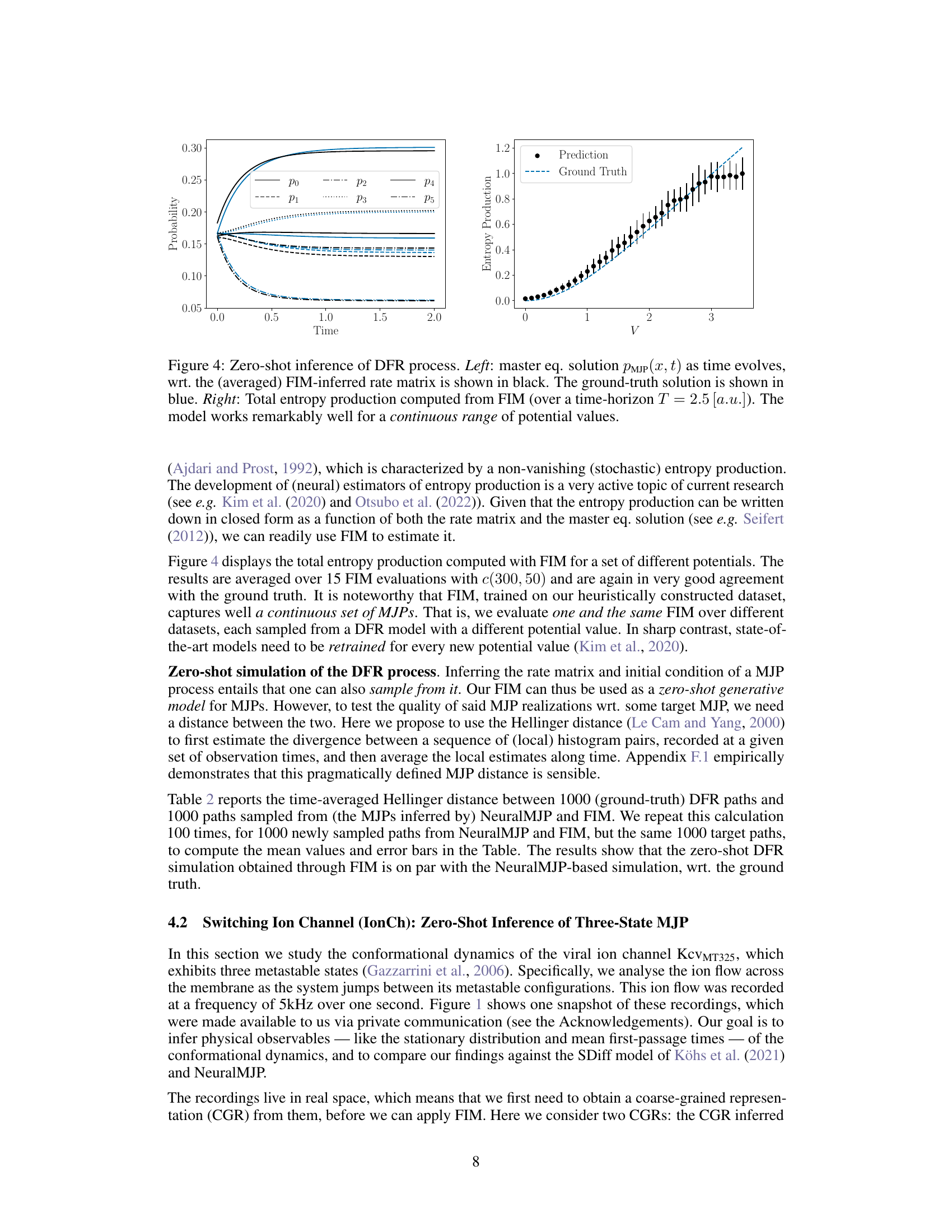
🔼 The left panel shows the time evolution of the probability distribution over the six states of the discrete flashing ratchet process. The black lines represent the prediction by the Foundation Inference Model (FIM), while the blue lines represent the ground truth. The right panel shows the total entropy production computed from the FIM’s prediction as a function of the potential value (V). Both plots demonstrate that FIM accurately infers the dynamics of the DFR process across a range of potential values.
read the caption
Figure 4: Zero-shot inference of DFR process. Left: master eq. solution PMJP(x, t) as time evolves, wrt. the (averaged) FIM-inferred rate matrix is shown in black. The ground-truth solution is shown in blue. Right: Total entropy production computed from FIM (over a time-horizon T = 2.5 [a.u.]). The model works remarkably well for a continuous range of potential values.
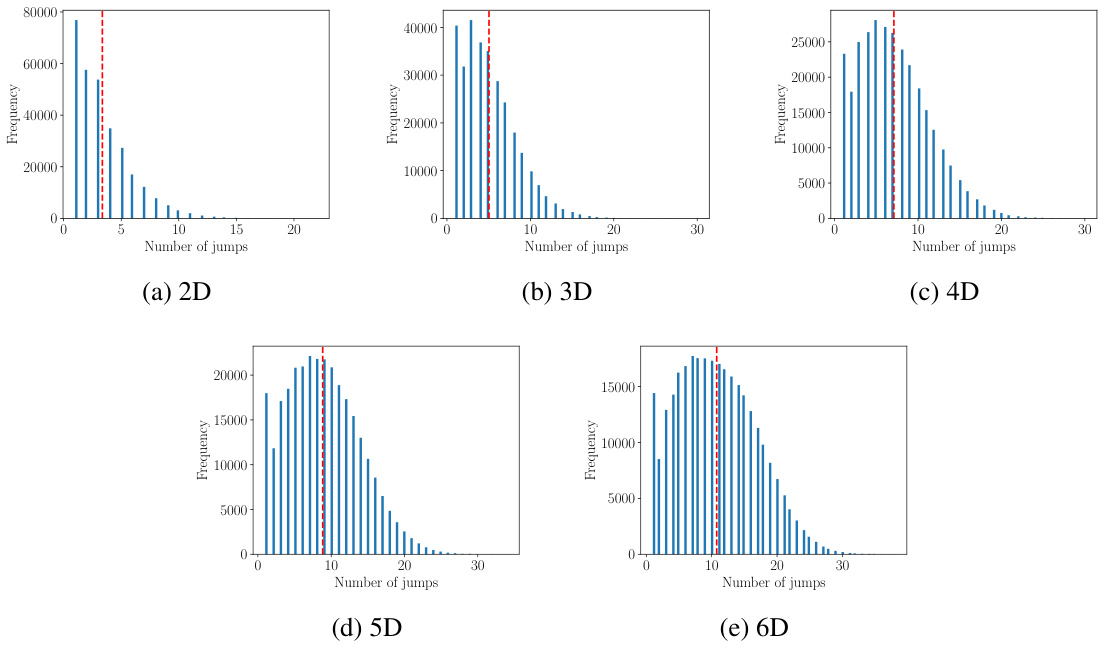
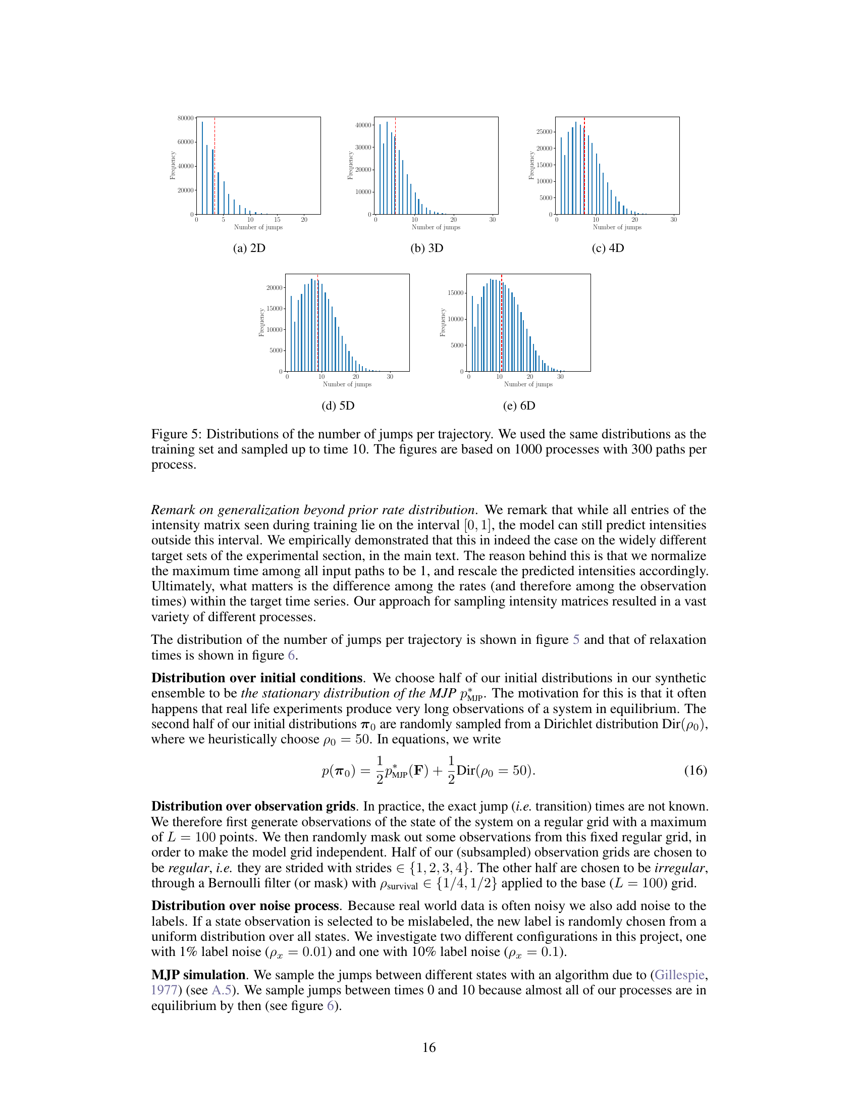
🔼 This figure shows the distribution of the number of jumps observed in 1000 simulated Markov jump processes (MJPs), each with 300 paths, up to time 10. The distributions are displayed for different state space dimensions (2D to 6D). The distributions are similar to those used in the training set, demonstrating the effectiveness of the data generation method in creating a representative dataset.
read the caption
Figure 5: Distributions of the number of jumps per trajectory. We used the same distributions as the training set and sampled up to time 10. The figures are based on 1000 processes with 300 paths per process.
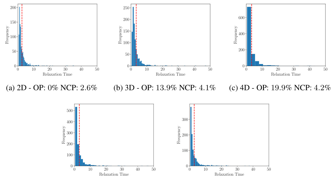
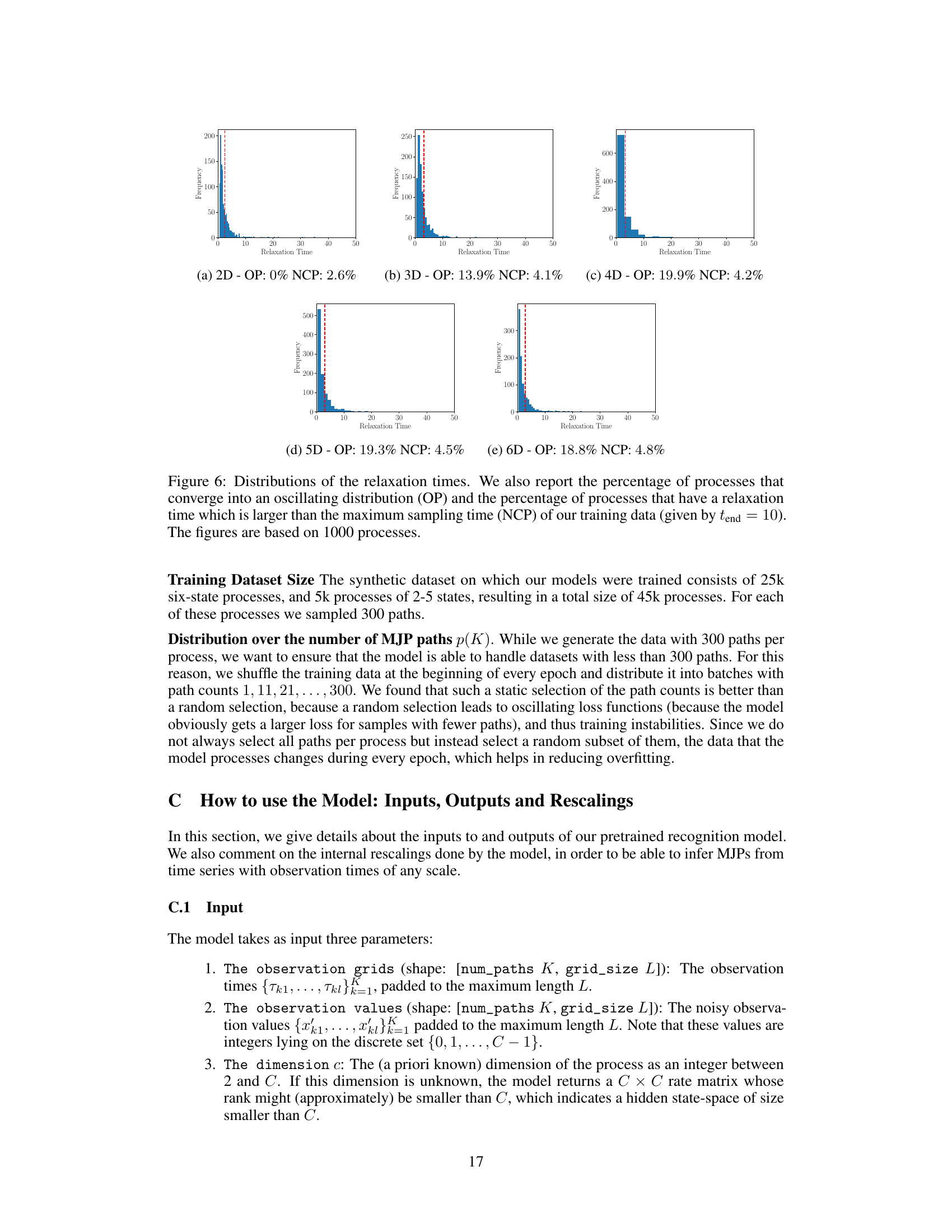
🔼 The figure shows the distributions of relaxation times for Markov jump processes with state spaces of different dimensions. The red dashed line indicates the maximum sampling time used during training. The percentages of processes that converge to oscillating distributions (OP) and those exceeding the maximum sampling time (NCP) are also provided for each dimensionality. The distributions illustrate the range of relaxation times observed in the simulated data.
read the caption
Figure 6: Distributions of the relaxation times. We also report the percentage of processes that converge into an oscillating distribution (OP) and the percentage of processes that have a relaxation time which is larger than the maximum sampling time (NCP) of our training data (given by tend = 10). The figures are based on 1000 processes.

🔼 This figure presents an ablation study evaluating the impact of different hyperparameter settings on the RMSE of the model. It shows how changes in the hidden size of the path encoder (ψ₁), the architecture size of ψ₁, and ψ₂, and the hidden size of the attention network (Ω₁) affect the model’s performance. The results suggest that the path encoder and its first feed-forward layer (φ₁) are particularly sensitive to hyperparameter changes, while the impact of the attention network is less pronounced.
read the caption
Figure 7: Impact of Hyperparameters on RMSE. The figure shows four line plots illustrating the effect of hyperparameters on model RMSE. The first plot shows RMSE increases with larger 41 hidden sizes, being lowest at 256. The second plot indicates lower RMSE with a larger 41 architecture size ([2x128]). The third plot shows minimal RMSE impact from 42 architecture size. The fourth plot shows RMSE stability across different Ω₁ hidden sizes, with slight variations based on 41. This highlights the importance of tuning 41 and 41 for optimal performance.

🔼 This figure shows the average Hellinger distance between the model’s predictions and the ground truth for different values of the potential V. The average Hellinger distance is computed using 100 histograms for each potential value. As expected, the distance decreases as the potential V approaches the target value of 1. The error bars represent the standard deviation of the Hellinger distances.
read the caption
Figure 8: Time-Average Hellinger distance for varying potentials on the DFR. The plot shows the Hellinger distance to a target dataset that was sampled from a DFR with V = 1 on a grid of 50 points between 0 and 2.5. The means and standard deviations were computed by sampling 100 histograms per dataset. As expected, the distance decreases as the voltage gets closer to the voltage of the target dataset. We also remark that the scale of the distances gets smaller as one takes more paths into account and converge to the distance of the solutions of the master equation.

🔼 This figure compares the clustering results of the Alanine Dipeptide dataset using two different methods: KMeans and NeuralMJP. It visually demonstrates how each method groups the data points into different clusters (representing different conformational states). The figure is crucial in the context of the paper because it shows how the choice of coarse-graining method (KMeans vs NeuralMJP) can influence the subsequent analysis and inference of Markov jump processes (MJPs). The differences in clustering observed in Figure 9 lead to differences in the learned MJP models, highlighting the impact of the preprocessing step on downstream inference results.
read the caption
Figure 9: Comparison of the classifications between KMeans (left) and NeuralMJP (right).

🔼 This figure shows two examples of time series data exhibiting jump processes. The left panel shows data from a discrete flashing ratchet process, illustrating the discrete jumps between states. The right panel shows a current signal from a viral potassium channel, also demonstrating jumps between different levels of activity. This figure highlights that seemingly different systems, after coarse-graining, can exhibit similar jump-process dynamics.
read the caption
Figure 1: Processes of very different nature (seem to) feature similar jump processes. Left: State values (blue circles) recorded from the discrete flashing ratchet process (black line). Right: Current signal (blue line) recorded from the viral potassium channel KcvMT35, together with one possible coarse-grained representation (black line).
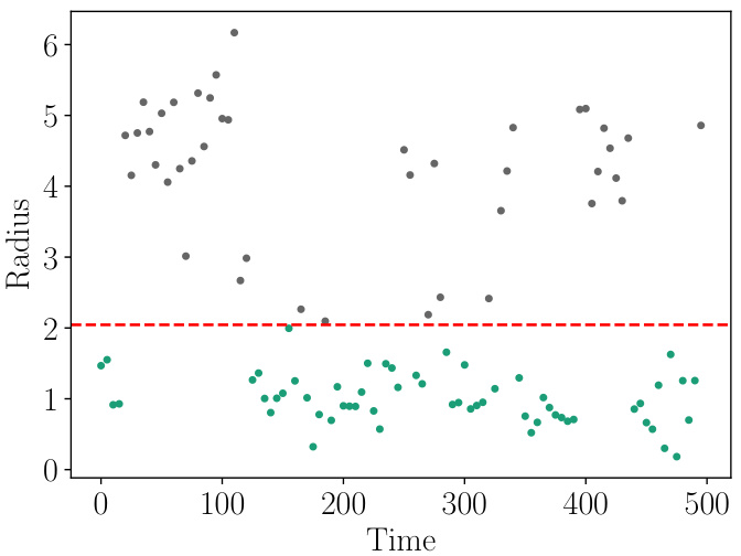
🔼 This figure shows the classification of a protein folding dataset into two states, Low and High, using a Gaussian Mixture Model (GMM). The GMM classifier learns a decision boundary close to a radius of 2. The plot likely displays the radius values on the y-axis and time or simulation steps on the x-axis. Each point represents a data point from the dataset, with different colors (or shapes) possibly indicating the Low and High states. This visualization helps understand how well the GMM classifier separates the two states based on the radius feature.
read the caption
Figure 11: Classification of the protein folding dataset into a Low and a High state. The GMM-Classifier has learned a decision boundary close to the radius 2.
More on tables

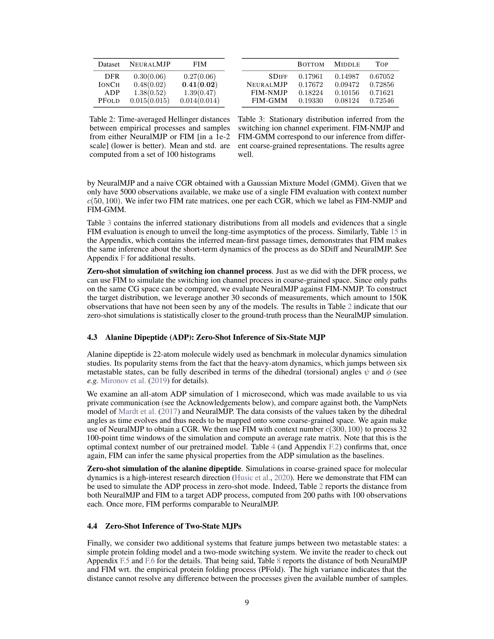
🔼 This table compares the performance of NeuralMJP and FIM by calculating the time-averaged Hellinger distance between the empirical processes and samples generated by each model. A lower Hellinger distance indicates better performance, meaning the model’s generated samples more closely resemble the actual empirical data. The mean and standard deviation are computed from 100 sets of histograms, providing a measure of variability and confidence in the results.
read the caption
Table 2: Time-averaged Hellinger distances between empirical processes and samples from either NeuralMJP or FIM [in a le-2 scale] (lower is better). Mean and std. are computed from a set of 100 histograms

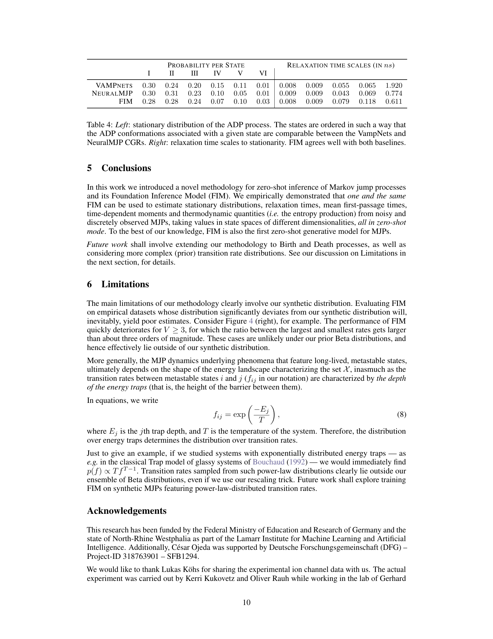
🔼 This table compares the stationary distributions and relaxation time scales obtained from three different models: VAMPNETS, NEURALMJP, and FIM, for the Alanine Dipeptide (ADP) process. The stationary distribution shows the probability of the system being in each of the six metastable states. The relaxation time scales represent the time it takes for the system to converge to its stationary distribution from different initial states. The table demonstrates that FIM’s results are in good agreement with the other two models.
read the caption
Table 4: Left: stationary distribution of the ADP process. The states are ordered in such a way that the ADP conformations associated with a given state are comparable between the VampNets and NeuralMJP CGRs. Right: relaxation time scales to stationarity. FIM agrees well with both baselines.
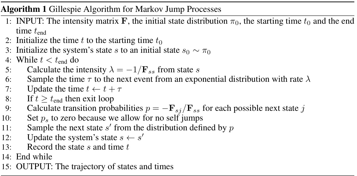
🔼 This table presents the time-averaged Hellinger distances, a measure of similarity between probability distributions, calculated between empirical processes and samples generated by two models: NeuralMJP and FIM. Lower values indicate better agreement between the models’ generated samples and the real data. The mean and standard deviation of the distances are calculated from 100 histogram comparisons for each dataset. The distances are scaled by 1e-2.
read the caption
Table 2: Time-averaged Hellinger distances between empirical processes and samples from either NeuralMJP or FIM [in a le-2 scale] (lower is better). Mean and std. are computed from a set of 100 histograms.

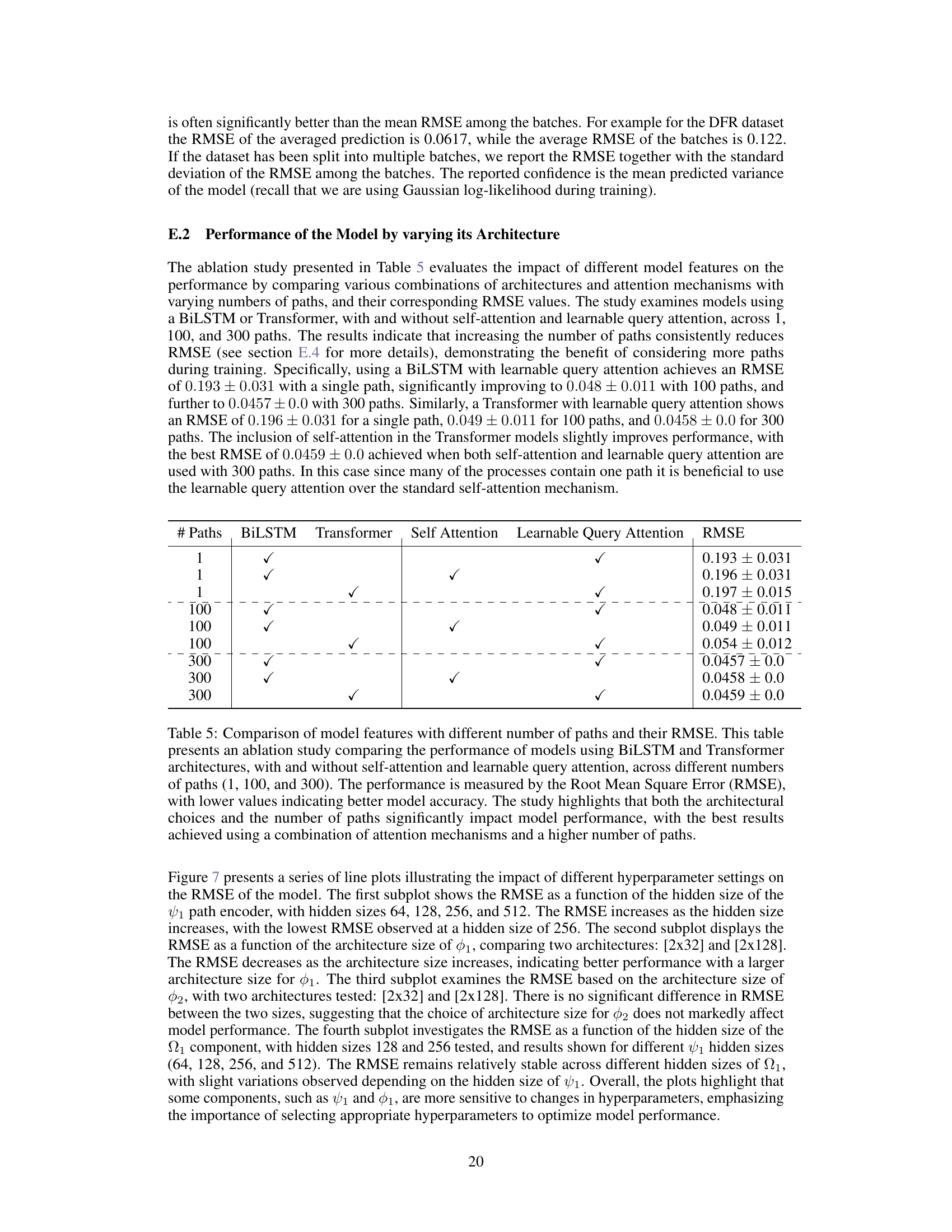
🔼 This table presents the ablation study by comparing the performance of different model architectures and attention mechanisms with varying numbers of paths. The results show that increasing the number of paths consistently reduces the RMSE, indicating that considering more paths during training improves accuracy. The best performance is achieved by using a BiLSTM or Transformer network with learnable query attention and a higher number of paths.
read the caption
Table 5: Comparison of model features with different number of paths and their RMSE. This table presents an ablation study comparing the performance of models using BiLSTM and Transformer architectures, with and without self-attention and learnable query attention, across different numbers of paths (1, 100, and 300). The performance is measured by the Root Mean Square Error (RMSE), with lower values indicating better model accuracy. The study highlights that both the architectural choices and the number of paths significantly impact model performance, with the best results achieved using a combination of attention mechanisms and a higher number of paths.

🔼 This table presents the results of evaluating two different Foundation Inference Models (FIMs), FIM-MJP 1% and FIM-MJP 10%, on synthetic datasets with varying levels of noise (1% and 10%). The models were trained on synthetic data with either 1% or 10% noise respectively. The table shows the root mean squared error (RMSE) for each model on each noise level. The RMSE is calculated as a weighted average across datasets with different numbers of states, which allows for better comparison of model performance across varying datasets.
read the caption
Table 6: Performance of FIM-MJP 1% and FIM-MJP 10% on synthetic datasets with different noise levels. We use a weighted average among the datasets with different numbers of states to compute a final RMSE.

🔼 This table compares the performance of two models on synthetic datasets with different numbers of states. The ‘Multi-State’ model was trained on datasets with a varying number of states (2-6), while the ‘6-State’ model was trained only on datasets with 6 states. The RMSE (Root Mean Square Error) and confidence values are reported for each model and number of states. Lower RMSE values indicate better performance.
read the caption
Table 7: Performance of the multi-state and six-state models (which has only been trained on processes with six states) on synthetic test sets with varying number of states

🔼 This table presents the results of an ablation study on the performance of the FIM-MJP model with different numbers of paths during evaluation on the Discrete Flashing Ratchet (DFR) dataset. It compares the Root Mean Square Error (RMSE) and confidence of the model using two different attention mechanisms: learnable query attention (LQ) and self-attention (SA). The table shows that increasing the number of paths generally improves the RMSE and confidence. However, it also shows that significantly exceeding the training range (300 paths) leads to poor performance, especially for the self-attention mechanism.
read the caption
Table 8: Performance of FIM-MJP 1% given varying number of paths during the evaluation on the DFR dataset with regular grid. (LQ) denotes learnable-query-attention (see section D.1), (SA) denotes self-attention.

🔼 This table presents the time-averaged Hellinger distances, a measure of similarity between probability distributions. It compares the distances between empirical processes (real-world data) and samples generated by two different models: NeuralMJP and FIM. Lower values indicate better model performance (i.e. a closer match between the model-generated data and the real data). The averages and standard deviations are calculated from 100 histogram comparisons.
read the caption
Table 2: Time-averaged Hellinger distances between empirical processes and samples from either NeuralMJP or FIM [in a le-2 scale] (lower is better). Mean and std. are computed from a set of 100 histograms.
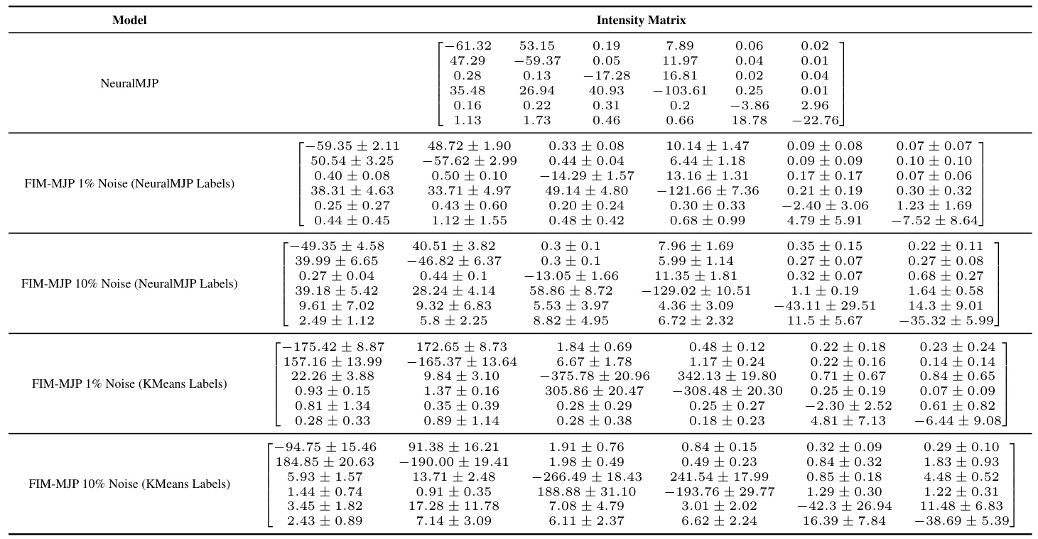
🔼 This table compares the performance of different models (NeuralMJP, FIM-MJP with 1% noise, and FIM-MJP with 10% noise) by calculating the time-averaged Hellinger distance between the model predictions and the target datasets. The datasets used include Alanine Dipeptide (ADP), Ion Channel, Protein Folding, and Discrete Flashing Ratchet (DFR). Lower Hellinger distance indicates better model performance. The results show that FIM-MJP performs comparably to NeuralMJP, even with the presence of noise. The high variance observed for the protein folding dataset is attributed to the models’ near-perfect predictions.
read the caption
Table 9: Comparison of the time-average Hellinger distances for various models. We used the same labels as NeuralMJP to make the results comparable. The errors are the standard deviation among 100 sampled histograms. The target datasets contain 200 paths for ADP, 1500 paths for Ion Channel, 2000 paths for Protein Folding and 1000 paths for the DFR. The distances are reported in a scale 1e-2. We remark that the high variance of the distances on the Protein Folding dataset is caused by the models performing basically perfect predictions, which causes the oscillations to be noise. We verified this claim by confirming that the distances of the predictions of the models are as small as the distance of the target dataset to additional simulated data.

🔼 This table compares the stationary distribution and relaxation time scales obtained from three different methods: VAMPNETS, NeuralMJP, and FIM. The left side shows the stationary distribution (probability of being in each state) for the alanine dipeptide (ADP) process, ensuring that the states are comparable across the different methods used for coarse-grained representation. The right side displays the relaxation times to stationarity, offering a measure of how quickly the system reaches a steady state. The results illustrate that the FIM model’s estimations are highly consistent with those produced by the other two methods.
read the caption
Table 4: Left: stationary distribution of the ADP process. The states are ordered in such a way that the ADP conformations associated with a given state are comparable between the VampNets and NeuralMJP CGRs. Right: relaxation time scales to stationarity. FIM agrees well with both baselines.

🔼 This table presents the time-averaged Hellinger distances, a measure of similarity between probability distributions, calculated between empirical processes (real-world data) and samples generated by two different models: NeuralMJP and FIM. Lower values indicate higher similarity, meaning the model’s generated samples more closely resemble the real-world data. The results are averaged over 100 histogram comparisons, with standard deviations provided to show the variability of the estimates.
read the caption
Table 2: Time-averaged Hellinger distances between empirical processes and samples from either NeuralMJP or FIM [in a le-2 scale] (lower is better). Mean and std. are computed from a set of 100 histograms
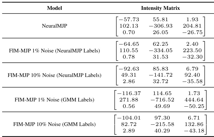
🔼 The table compares the intensity matrices obtained from different models for the ion channel dataset. The models compared include NeuralMJP, and FIM-MJP with 1% and 10% noise levels, using both NeuralMJP labels and GMM labels. Due to the small size of the dataset, error bars cannot be reliably calculated, making comparison less precise than for other datasets with more samples.
read the caption
Table 13: Comparison of intensity matrices for the ion channel dataset. We cannot report error bars here because the dataset is so small that it gets processed in a single batch.

🔼 This table presents the stationary distributions obtained from different models for the switching ion channel experiment. The results show that the FIM model, even without fine-tuning, achieves results comparable to other state-of-the-art methods. The FIM-NMJP and FIM-GMM results represent inferences from two different coarse-grained representations of the data, demonstrating the model’s robustness to different preprocessing choices.
read the caption
Table 3: Stationary distribution inferred from the switching ion channel experiment. FIM-NMJP and FIM-GMM correspond to our inference from different coarse-grained representations. The results agree well.

🔼 This table compares the mean first-passage times (MFPTs) for transitions between three states of a switching ion channel model, as predicted by various methods: Köhs et al. (2021), NeuralMJP, and the proposed FIM (Foundation Inference Model) with different noise levels and label types (NeuralMJP or GMM). MFPT values represent the average time taken for the system to transition from one state to another. The table allows assessing the accuracy of the FIM’s predictions compared to established methods.
read the caption
Table 15: Mean first-passage times of the predictions of various models on the Switching Ion Channel dataset. We compare against (Köhs et al., 2021) and NeuralMJP (Seifner and Sánchez, 2023). Entry j in row i is mean first-passage time of transition i→j of the corresponding model.

🔼 This table compares the intensity matrices obtained from the ground truth, FIM-MJP with 1% noise, and FIM-MJP with 10% noise for the Discrete Flashing Ratchet (DFR) process using an irregular grid. Each model’s matrix is shown, providing a comparison of the estimated transition rates between states with varying levels of noise in the observation data.
read the caption
Table 16: Comparison of intensity matrices for the DFR dataset on the irregular grid.

🔼 This table presents a comparison of the stationary distributions obtained from various models on the protein folding dataset. The models compared include MARDT ET AL. (2017), NEURALMJP, and different versions of FIM-MJP (with varying noise levels and labeling methods). The stationary distribution is represented by the probabilities of being in a Low or High state, reflecting the folded and unfolded conformations of the protein. The table helps assess the accuracy of different models in predicting the equilibrium state of the protein-folding process.
read the caption
Table 18: Stationary distribution of the model predictions on the protein folding dataset

🔼 This table compares the predicted transition rates between the low and high states for different models on a protein folding dataset. The models include NeuralMJP and various versions of the FIM-MJP model with differing noise levels (1% and 10%) and data labeling methods (NeuralMJP labels and GMM labels). The transition rates are presented as Low STD → HIGH STD and HIGH STD → LOW STD, representing the transition probabilities from a low standard deviation state to a high standard deviation state and vice versa.
read the caption
Table 17: Predicted transition rates on the protein folding dataset
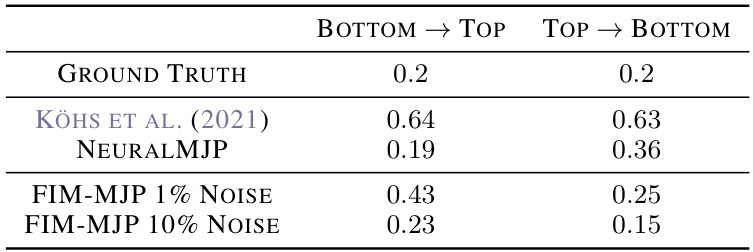
🔼 This table presents the transition rates for a two-mode switching system. The results are compared to those from Köhs et al. (2021) and NeuralMJP. Error bars are not reported because the dataset size is too small for reliable statistical measures.
read the caption
Table 19: Two-Mode Switching System transition rates. We do not report error bars here because the dataset is so small that it runs in a single batch.

🔼 This table presents the results of comparing the performance of the proposed FIM and the NeuralMJP model. The comparison is done based on the time-averaged Hellinger distance between the empirical processes and samples generated by each model. Lower values in the table indicate better performance. The mean and standard deviation are computed over 100 histograms for each comparison.
read the caption
Table 2: Time-averaged Hellinger distances between empirical processes and samples from either NeuralMJP or FIM [in a le-2 scale] (lower is better). Mean and std. are computed from a set of 100 histograms
Full paper#
