TL;DR#
Label Distribution Learning (LDL) is valuable for handling label polysemy in machine learning, but accurately quantifying label distributions is costly. Current methods rely on binary annotations from experts, which can be inefficient and prone to errors, especially when dealing with ambiguous instances. This paper addresses these challenges by introducing a novel approach that uses ternary labels (‘definitely relevant’, ‘uncertain’, ‘definitely irrelevant’).
The researchers propose predicting label distributions directly from these ternary labels. They introduce a new probability distribution called CateMO, designed to model the mapping from label description degrees to ternary labels. This distribution serves as a loss function and ensures that the model’s predictions respect the monotonicity and ordinality inherent in the ternary labeling scheme. Through theoretical analysis and experiments, they demonstrate that their approach reduces annotation costs and improves accuracy compared to existing methods using binary labels.
Key Takeaways#
Why does it matter?#
This paper is important because it introduces a novel approach to label distribution learning (LDL), a crucial task in many machine learning applications. By using ternary labels instead of traditional binary labels, it significantly improves annotation efficiency and accuracy. The proposed CateMO distribution provides a robust framework for modeling the relationship between label description degrees and ternary labels, offering a more nuanced and informative representation of label polysemy. This work opens new avenues for research in LDL and related areas.
Visual Insights#

🔼 This figure illustrates the challenges of binary annotation in multi-label learning. A facial image is shown, and the task is to determine which emotions are present. While some emotions (e.g., ‘Sad’, ‘Happy’) are clearly absent, others (e.g., ‘Surprise’, ‘Fear’) present more ambiguity. The annotation scheme shows how using binary labels (+1 or -1) can be inaccurate in such cases, making a ’ternary label’ approach with a third option (0 for ‘uncertain’) much more accurate. This ambiguity highlights the motivation for using ternary labels instead of binary labels.
read the caption
Figure 1: An annotation from JAFFE dataset [18].

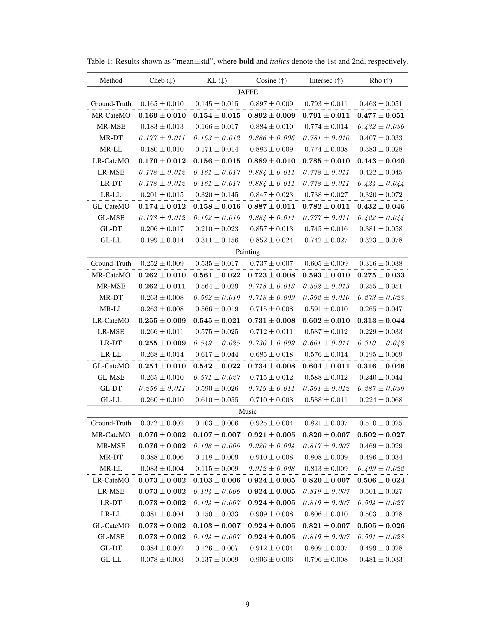
🔼 This table presents the performance comparison of different label distribution prediction methods on three datasets: JAFFE, Painting, and Music. The methods are categorized into those using binary labels directly and those that adapt to ternary labels using three different strategies: data transformation (DT), mean squared error (MSE), and the proposed CateMO distribution. For each method, the table shows the mean and standard deviation of five common evaluation metrics: Chebyshev distance (Cheb), Kullback-Leibler divergence (KL), cosine similarity (Cosine), intersection (Intersec), and Spearman’s rank correlation coefficient (Rho). Lower values for Cheb and KL, and higher values for Cosine, Intersec, and Rho indicate better performance. The ground-truth results are also included as a baseline.
read the caption
Table 1: Results shown as “mean±std”, where bold and italics denote the 1st and 2nd, respectively.
In-depth insights#
Ternary Label Power#
The concept of “Ternary Label Power” suggests an approach to label data that moves beyond the traditional binary (0/1) classification. A ternary system (e.g., -1, 0, +1 representing definitely irrelevant, uncertain, and definitely relevant) offers a more nuanced representation of the complex relationships between data points and labels. This added granularity can reduce annotation ambiguity and potentially improve model accuracy, especially when dealing with complex or ambiguous datasets. The challenge lies in designing algorithms that effectively leverage the uncertainty inherent in the ‘0’ label, perhaps through probabilistic modeling or by incorporating uncertainty directly into the loss function. While ternary labels require more annotation effort upfront, the potential for improved model accuracy and robustness could be significant, especially for applications where high accuracy is essential, and uncertainty in the data is unavoidable. Careful selection of the threshold values separating the three label states would be crucial for practical implementation.
CateMO Modeling#
The proposed CateMO (Categorical distribution with Monotonicity and Orderliness) model offers a novel approach to addressing the limitations of traditional binary label annotations in label distribution learning. By incorporating a ternary annotation scheme (positive, negative, uncertain), CateMO directly models the mapping between label description degrees and ternary labels. This is a significant improvement over existing methods that rely on binary labels, which may misrepresent the ambiguity inherent in many real-world label assignments. CateMO’s theoretical foundation rests on assumptions of probability monotonicity and orderliness, which ensure that the model’s predictions are coherent and interpretable. The model’s flexibility and adaptability, as demonstrated by its use within existing label enhancement frameworks, is a key strength, potentially improving accuracy and efficiency in label distribution learning tasks. The experimental validation of CateMO’s effectiveness further underscores its potential value as a powerful tool in scenarios where precise label quantification is difficult or costly.
Error Approximation#
The concept of ‘Error Approximation’ in a research paper is crucial for evaluating the accuracy and reliability of a model or method. It involves quantifying the difference between the model’s predictions and the actual, true values. A good error approximation method should be accurate, reflecting the true error, robust, insensitive to outliers or noise, and interpretable, providing insights into the nature and sources of errors. Different error metrics are used depending on the context—mean squared error (MSE) for regression tasks, cross-entropy for classification. The paper likely discusses the choice and justification of a specific error metric. It is essential to show that the chosen approximation method is valid and avoids bias. A key aspect often explored is comparing different approximation methods, potentially including simpler, faster approximations versus more complex, computationally expensive ones. A rigorous evaluation would analyze the trade-offs between accuracy and computational cost. Furthermore, examining how the error approximation changes under various conditions (e.g., with increased data, different model parameters) is vital to show the method’s reliability and limitations.
Experimental Design#
An effective experimental design is crucial for validating the claims made in the research paper. It should begin with a clear articulation of the research question and hypotheses. The selection of datasets needs careful consideration, ensuring they are representative of the problem domain and diverse enough to avoid overfitting. The choice of comparison algorithms is critical; selecting methods that are established and directly comparable is important to avoid biased results. A robust evaluation methodology is also necessary, which includes a thorough description of the metrics used and the statistical significance tests performed. The parameter configurations of the chosen methods must be explicitly outlined, and the process for hyperparameter tuning should be transparently documented to ensure the reproducibility of the experimental results. Finally, the experimental design should encompass sufficient repetitions and a rigorous analysis of the results to draw sound conclusions.
Future Enhancements#
The research paper’s “Future Enhancements” section could explore several promising avenues. Extending the ternary labeling scheme to incorporate nuanced uncertainty levels beyond the simple ‘uncertain’ category would provide a more granular representation of expert knowledge. Another key area would be to investigate more sophisticated models for the mapping between label description degrees and ternary labels, potentially incorporating advanced probabilistic techniques or deep learning approaches for improved prediction accuracy. Further research could delve into developing robust methods for handling imbalanced datasets, a common challenge in label distribution learning. Finally, a crucial direction for future work is conducting extensive cross-dataset validation to assess the generalizability of the proposed framework. The effectiveness of CateMO in diverse real-world settings needs further investigation to build trust in its reliability and potential impact.
More visual insights#
More on figures
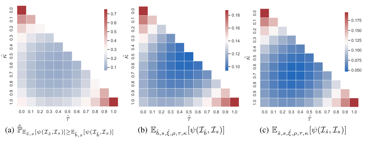
🔼 This figure presents a quantitative comparison of the approximation error between ternary and binary labels. It shows the distributions of the expected approximation error (EAE) for both ternary and binary labels across various parameter ranges (τ, κ, ξ, ρ). The figure also illustrates the approximate proportion of cases where the ternary label’s EAE is greater than that of the binary label. This visually demonstrates the superiority of ternary labels in approximating the ground truth label description degrees.
read the caption
Figure 2: Distributions of the values of PEs,s[ψ(Is,Is)]≥Eô,s[ψ(Iô,Is)], Eô,s,ξ,ρ,τ,κ[ψ(Iô,Is)], and Eŝ,s,ξ,ρ,τ,κ[ψ(Iŝ,Is)] over [τ,κ], where Eô,s,ξ,ρ,τ,κ[ψ(Iô,Is)] and Eŝ,s,ξ,ρ,τ,κ[ψ(Iŝ,Is)] (which are defined in Equation (7)) measures the average EAE of binary labels and ternary labels, respectively; PEs,s[ψ(Is,Is)]≥Eô,s[ψ(Iô,Is)] is defined in Equation (8), which measures the approximate proportion of cases where the ternary label is inferior to the binary label for different [τ,κ,ξ,ρ].

🔼 This figure visualizes the conditions derived in Theorem 1, which ensures the superiority of ternary labels over binary labels in approximating ground-truth label description degrees. It shows the overlapping area of conditions where ternary labels outperform binary labels, highlighting the superiority of the ternary labeling approach for improved accuracy in label distribution prediction. The x-axis and y-axis represent the parameters ↑ and κ which defines the boundary of intervals for label description degree z.
read the caption
Figure 3: The visualization of ↑ ≤ k and ( − 1)² + ( − 1)² ≤ 4
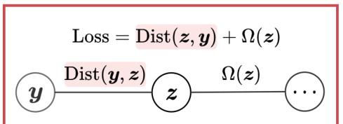
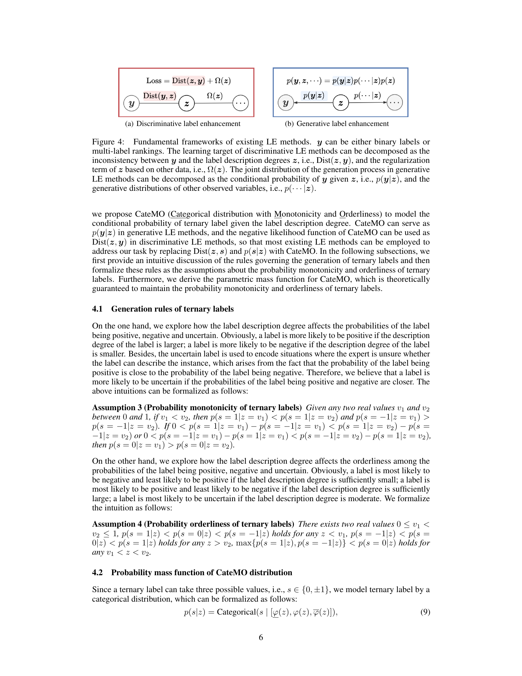
🔼 This figure illustrates the fundamental frameworks of existing Label Enhancement (LE) methods. It shows two main approaches: discriminative and generative. Discriminative LE focuses on minimizing the inconsistency between easily accessible labels (y) and label description degrees (z), while also considering regularization terms (Ω(z)). Generative LE models the generation process by describing the joint distribution of labels (y), z, and other variables. The figure highlights how different LE methods handle the relationship between y and z.
read the caption
Figure 4: Fundamental frameworks of existing LE methods. y can be either binary labels or multi-label rankings. The learning target of discriminative LE methods can be decomposed as the inconsistency between y and the label description degrees z, i.e., Dist(z, y), and the regularization term of z based on other data, i.e., Ω(z). The joint distribution of the generation process in generative LE methods can be decomposed as the conditional probability of y given z, i.e., p(y|z), and the generative distributions of other observed variables, i.e., p(···|z).
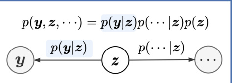
🔼 This figure illustrates the fundamental frameworks of existing Label Enhancement (LE) methods, categorizing them into discriminative and generative approaches. Discriminative LE directly models the relationship between accessible labels (y) and label description degrees (z) using a loss function (Dist(z,y)) and regularization (Ω(z)). Generative LE, in contrast, models the joint probability distribution of y, z, and other variables, decomposing it into p(y|z), p(···|z), and p(z).
read the caption
Figure 4: Fundamental frameworks of existing LE methods. y can be either binary labels or multi-label rankings. The learning target of discriminative LE methods can be decomposed as the inconsistency between y and the label description degrees z, i.e., Dist(z, y), and the regularization term of z based on other data, i.e., Ω(z). The joint distribution of the generation process in generative LE methods can be decomposed as the conditional probability of y given z, i.e., p(y|z), and the generative distributions of other observed variables, i.e., p(···|z).

🔼 This figure visualizes the probability distributions p(s|z) of the CateMO model for different parameter settings. The x-axis represents the label description degree (z), which is a continuous value between 0 and 1 representing how strongly a label describes an instance. The y-axis shows the probability p(s|z), representing the probability of assigning each of the three ternary labels (-1, 0, 1) given the label description degree z. Each subplot shows the probability curves for the three ternary labels for a different set of parameters (λ, λ, λ, x), illustrating how the shape of the distribution changes depending on parameter values. The parameter λ represents the weight for the negative label, λ for the positive label, and λ for the uncertain label. x is a parameter that influences the transition point between negative and positive labels.
read the caption
Figure 5: p(s|z) on different parameters. The horizontal and vertical axes denote the label description degree z and the probability p(s|z) defined by Equation (9) and Equation (10), respectively.

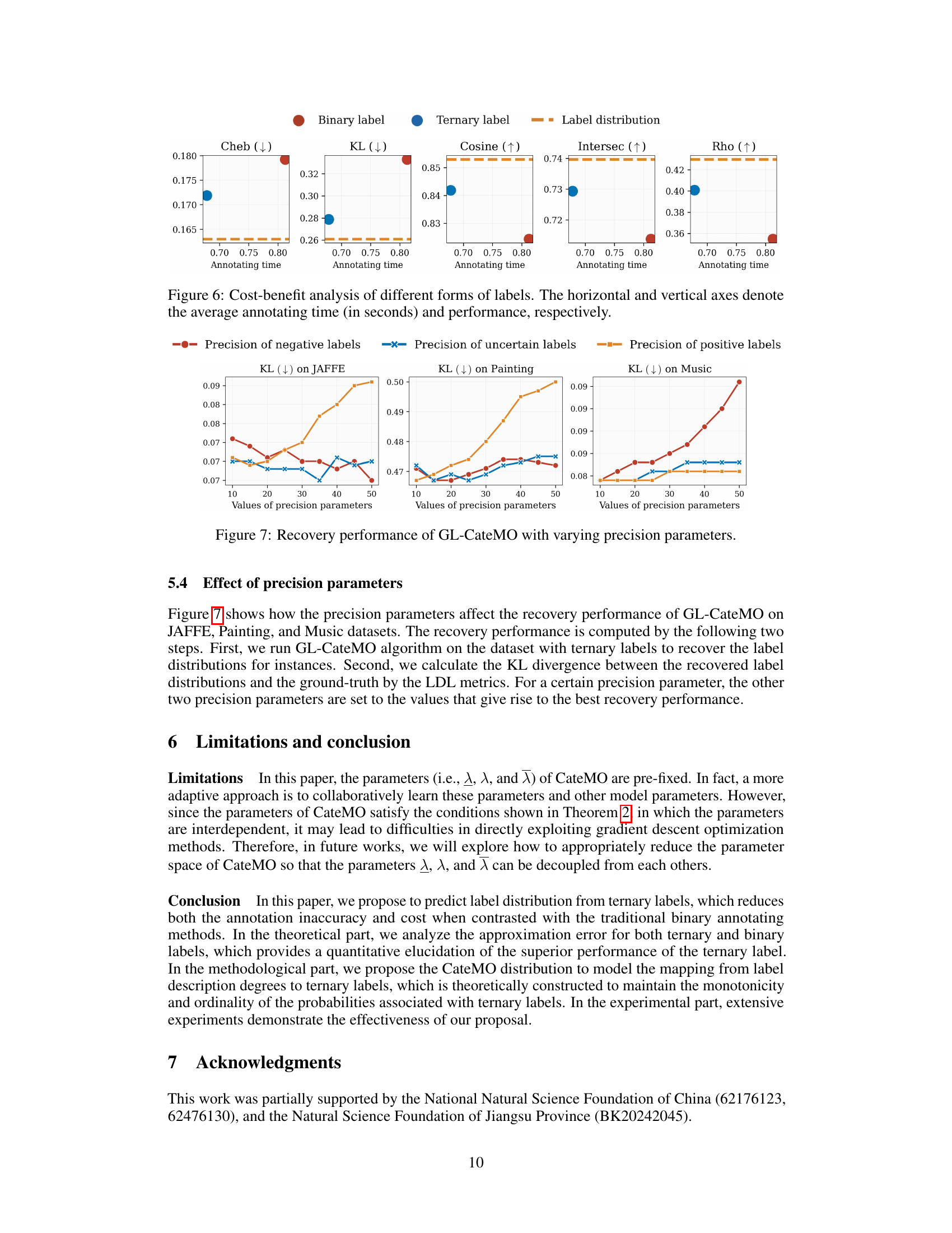
🔼 This figure displays a cost-benefit analysis comparing the use of binary labels versus ternary labels in a label distribution learning task. The x-axis represents the average time spent annotating each label, while the y-axis shows the performance achieved using different label types. The graph demonstrates that using ternary labels (which allows for uncertain annotations) results in superior performance and requires less annotation time compared to binary labels. This highlights the effectiveness of the proposed ternary annotation approach, balancing both efficiency and accuracy.
read the caption
Figure 6: Cost-benefit analysis of different forms of labels. The horizontal and vertical axes denote the average annotating time (in seconds) and performance, respectively.

🔼 This figure shows how the precision parameters affect the recovery performance of GL-CateMO on JAFFE, Painting, and Music datasets. The recovery performance is computed in two steps: first, running GL-CateMO to recover label distributions; second, calculating KL divergence between recovered and ground-truth distributions. For a given precision parameter, the other two are set to values resulting in best recovery performance. The x-axis represents the values of precision parameters, and the y-axis represents the KL divergence (lower is better). Three subplots display results for each dataset.
read the caption
Figure 7: Recovery performance of GL-CateMO with varying precision parameters.
Full paper#


