TL;DR#
Deep learning optimization is complex due to non-convex objective functions. Understanding optimization dynamics is crucial, particularly the relationship between sharpness (Hessian’s largest eigenvalue) and learning rate. Prior work has shown that sharpness should ideally remain below 2/η to avoid divergence during training; however, neural networks often operate at the edge of stability, challenging this notion.
This paper focuses on deep linear networks for univariate regression. The authors demonstrate that although minimizers can have arbitrarily high sharpness, there’s a lower bound that scales linearly with depth. They then analyze gradient flow (the limit of gradient descent with vanishing learning rate) to reveal an implicit regularization towards flatter minima: the sharpness of the minimizer is bound by a constant times the depth-dependent lower bound, independent of network width. This is shown for both small and residual initializations.
Key Takeaways#
Why does it matter?#
This paper is vital for researchers in deep learning optimization because it offers novel insights into the implicit regularization mechanisms of deep linear networks. The findings challenge conventional wisdom on how these networks avoid overfitting and provide a quantitative understanding of the relationship between learning rate, initialization, depth, and sharpness. This opens new avenues for designing more efficient training algorithms and improving the generalization capabilities of deep neural networks. It is directly relevant to current research trends on optimization dynamics and the implicit bias of deep learning models.
Visual Insights#

🔼 This figure shows the results of training a deep linear network on a univariate regression task using different learning rates and initialization scales. Plot (a) displays the squared distance of the trained network to the optimal regressor, revealing a critical learning rate below which training succeeds, independent of the initialization scale. Plot (b) illustrates the sharpness (largest eigenvalue of the Hessian) at initialization and after training, highlighting that training is possible even when initializing beyond the 2/η threshold. Plots (c) and (d) showcase the evolution of the squared distance to the optimal regressor and sharpness during training, demonstrating training dynamics under different conditions.
read the caption
Figure 1: Training a deep linear network on a univariate regression task with quadratic loss. The weight matrices are initialized as Gaussian random variables, whose standard deviation is the x-axis of plots 1a and 1b. Experimental details are given in Appendix C.

🔼 The table shows the number of gradient steps and the number of repetitions performed for different learning rates in the experiments for Figure 1 of the paper. The setup uses a Gaussian initialization of weight matrices where the x-axis in the plots represents the standard deviation of the entries. The table clarifies the experimental parameters used in the experiments generating the results shown in Figure 1.
read the caption
Details of Figure 1. We consider a Gaussian initialization of the weight matrices, where the scale of the initialization (x-axis of some the graphs) is the standard deviation of the entries. All weight matrices are d × d, except the last one which is 1 × d. The square distance to the optimal regressor corresponds to ||Wprod - w*||2. The largest eigenvalue of the Hessian is computed by a power iteration method, stopped after 20 iterations. In Figures 1a and 1b, the 95% confidence intervals are plotted. The number of gradient steps and number of independent repetitions depend on the learning rate, and are given below.
In-depth insights#
Implicit Regularization#
Implicit regularization in neural networks is a phenomenon where the training dynamics, even without explicit regularization terms, lead to solutions with desirable properties like generalization. Deep learning’s success hinges on this implicit bias, which often favors flat minima, low sharpness, and specific weight structures. The paper investigates this by analyzing deep linear networks for regression, revealing an implicit regularization towards flat minima despite the possibility of sharp minima existing. This is shown through gradient flow analysis, revealing that the sharpness of the minimizer is linked to the depth and data covariance, showcasing a controlled sharpness irrespective of network size. The results offer valuable insights into neural network optimization, hinting at a fundamental mechanism that steers training towards generalization-friendly solutions beyond the commonly understood effects of stochasticity and explicit regularization.
Sharp Minima Bounds#
The concept of sharpness, often represented as the largest eigenvalue of the Hessian matrix at a minimum, is crucial in understanding the generalization ability and optimization dynamics of neural networks. Research into sharp minima bounds investigates the range of possible sharpness values at optimal solutions. Lower bounds on sharpness often highlight inherent limitations in the optimization landscape, indicating that finding extremely flat minima might be impossible, even with sophisticated optimization techniques. Upper bounds, conversely, might suggest implicit regularization effects that prevent optimization from diverging into regions of excessively high sharpness. The interplay between these bounds, particularly in the context of factors like network depth and data properties, provides insights into how neural networks learn and generalize. Analyzing the behavior of gradient flow or gradient descent algorithms in relation to these bounds sheds light on the implicit biases of these methods and their effect on the final model’s characteristics. Furthermore, understanding how factors such as initialization strategies and learning rates affect sharpness bounds offers valuable guidance for training robust and generalizable neural networks.
Gradient Flow Dynamics#
Gradient flow dynamics, a continuous-time analog of gradient descent, offers valuable insights into neural network training. Analyzing gradient flow helps uncover implicit regularization mechanisms, shedding light on why neural networks generalize well despite their non-convex nature. Convergence properties of gradient flow are crucial; proving convergence guarantees under specific conditions enhances our understanding of training stability. Furthermore, studying the gradient flow reveals insights into the geometry of the loss landscape, such as the identification of flat minima that are associated with better generalization. Understanding the dynamics allows researchers to potentially design improved training algorithms and better initialization strategies. Characterizing the sharpness (Hessian’s largest eigenvalue) of the minimizers found through gradient flow is particularly important as sharpness relates to generalization and training stability.
Init. Schemes Compared#
A comparative analysis of initialization schemes is crucial for understanding deep learning dynamics. The heading ‘Init. Schemes Compared’ suggests an investigation into how different initialization strategies impact optimization, generalization, and the propensity for reaching flat minima. This could involve comparing small-scale initialization, where weights start near zero, to large-scale initialization, where they begin with larger magnitudes. The study might examine how these approaches affect the sharpness of minima, the convergence speed of gradient descent, and the final model’s generalization performance. Residual initialization, a technique utilizing residual connections to add stability, could also be included as a third scheme, contrasting its behavior with the others. The section would likely present both theoretical analyses, comparing the minimum achievable sharpness or convergence bounds across methods, and empirical results, showing the performance of each initialization on specific tasks and datasets. Overall, such a comparison would provide valuable insights into the implicit regularization properties of various initialization methods and their effect on deep learning outcomes.
Future Research#
Future research directions stemming from this work on implicitly regularized deep linear networks could explore several promising avenues. Extending the analysis to non-linear networks is crucial, as the theoretical elegance of linear models does not always translate to the complex dynamics of their non-linear counterparts. Investigating the influence of different activation functions and network architectures would be key. A deeper study of the interplay between sharpness, generalization, and the choice of learning rate is also warranted, potentially moving beyond the overdetermined regression setting analyzed here. The observed implicit regularization suggests connections to other regularization techniques, which should be investigated through both theoretical and empirical means. The algorithm’s behavior under different data distributions and noise models would provide a more comprehensive assessment of its robustness and practical applicability. Finally, exploring the scaling properties of the algorithm with respect to depth and width would provide further insights into its computational efficiency and limits.
More visual insights#
More on figures

🔼 This figure visualizes the training of a deep linear network on a univariate regression task using a quadratic loss function. The weight matrices are initialized with Gaussian random variables. The plots (a) and (b) show the relationship between the initialization scale (standard deviation of the Gaussian random variables) and the training results, showing the squared distance of the trained network from the optimal regressor and the sharpness (largest eigenvalue of the Hessian) at initialization and after training. Plots (c) and (d) illustrate the training dynamics (evolution of the squared distance and sharpness over training steps) for different learning rates to demonstrate the concept of the ’edge of stability’.
read the caption
Figure 1: Training a deep linear network on a univariate regression task with quadratic loss. The weight matrices are initialized as Gaussian random variables, whose standard deviation is the x-axis of plots 1a and 1b. Experimental details are given in Appendix C.
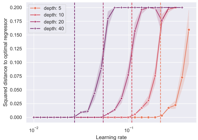
🔼 This figure shows the relationship between the learning rate and the squared distance to the optimal regressor for various depths of the neural network. The dashed vertical lines indicate the theoretical threshold of the learning rate. The results confirm that for a given depth, successful training occurs only when the learning rate is below the threshold.
read the caption
Figure 2: Squared distance of the trained network to the empirical risk minimizer, for various learning rates and depth. For each depth, learning succeeds if the learning rate is below a threshold, which corresponds to the theoretical value 2 ~ (||w*||32- La)−¹ of Theorem 1 (dashed vertical line).

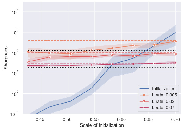
🔼 This figure shows the probability of divergence of the gradient descent algorithm for training deep linear networks for regression, using a Gaussian initialization of the weight matrices. The x-axis represents the scale of the initialization (standard deviation of Gaussian random variables), and the y-axis represents the probability of divergence. Different lines correspond to different learning rates. The plot reveals that for a fixed learning rate, there is a critical scale of initialization beyond which the network fails to learn (diverges). This critical scale depends on the learning rate; larger learning rates lead to divergence at smaller initialization scales.
read the caption
Figure 3: Probability of divergence of gradient descent for a Gaussian initialization of the weight matrices, depending on the initialization scale and the learning rate.

🔼 The figure shows the results of training deep linear networks on a univariate regression task. Plots (a) and (b) show the relationship between the initialization scale (standard deviation of Gaussian random variables used for initialization) and the learning rate’s effect on the training success and sharpness (largest eigenvalue of the Hessian) after training. Plot (c) shows a training run where the learning rate is below the critical value (no edge of stability), and (d) shows a run where the learning rate is above this value (edge of stability). The results illustrate the paper’s main findings of implicit regularization towards flat minima and a linear relationship between depth and minimal sharpness.
read the caption
Figure 1: Training a deep linear network on a univariate regression task with quadratic loss. The weight matrices are initialized as Gaussian random variables, whose standard deviation is the x-axis of plots 1a and 1b. Experimental details are given in Appendix C.

🔼 This figure shows the probability that the gradient descent diverges during training of a deep linear network for regression. The x-axis represents the scale of the Gaussian initialization of the weight matrices, while the different lines represent different learning rates. As the learning rate increases, the probability of divergence also increases, and for higher learning rates, divergence becomes more likely even with smaller initialization scales. The plot highlights the impact of the interplay between learning rate and initialization scale on the success of training.
read the caption
Figure 3: Probability of divergence of gradient descent for a Gaussian initialization of the weight matrices, depending on the initialization scale and the learning rate.
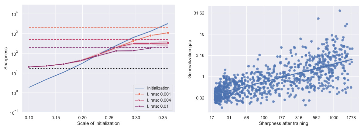
🔼 This figure shows the results of experiments performed on a deep linear network with a degenerate data covariance matrix (number of data points less than the dimension of the data). Panel (a) displays how sharpness at initialization and after training varies with the initialization scale for different learning rates. A key observation is a similar connection between learning rate, initialization scale, and sharpness to what was observed in the case of a full-rank data matrix. Panel (b) illustrates the relationship between generalization performance (generalization gap) and sharpness after training, exhibiting a positive correlation (linear regression has a slope of 0.42).
read the caption
Figure 6: Experiment with a deep linear network and a degenerate data covariance matrix, where the number of data n is less than the dimension d.
🔼 This figure shows the results of training deep linear networks on a univariate regression task. The x-axis represents the scale of the Gaussian initialization of the weight matrices (standard deviation). Plot (a) displays the squared distance of the trained network to the optimal regressor for various learning rates and initialization scales. Plot (b) shows the sharpness (largest eigenvalue of the Hessian) at initialization and after training, again for various learning rates and initialization scales. Plots (c) and (d) show the evolution during training of the squared distance to the optimal regressor and sharpness for specific learning rates and initialization scales. These plots illustrate the relationship between learning rate, initialization scale, and the sharpness of the resulting network minima. The plot helps explain the existence of a critical learning rate above which the network fails to train, a phenomenon that does not depend on the initial scale.
read the caption
Figure 1: Training a deep linear network on a univariate regression task with quadratic loss. The weight matrices are initialized as Gaussian random variables, whose standard deviation is the x-axis of plots 1a and 1b. Experimental details are given in Appendix C.
More on tables

🔼 This table details the experimental setup used to generate Figure 1 in the paper. It specifies the hyperparameters used (learning rate, number of steps, number of repetitions) for different learning rates. It also explains how the key metrics (squared distance to optimal regressor and sharpness) were computed.
read the caption
Details of Figure 1. We consider a Gaussian initialization of the weight matrices, where the scale of the initialization (x-axis of some the graphs) is the standard deviation of the entries. All weight matrices are d × d, except the last one which is 1 × d. The square distance to the optimal regressor corresponds to ||Wprod - w*||2. The largest eigenvalue of the Hessian is computed by a power iteration method, stopped after 20 iterations. In Figures 1a and 1b, the 95% confidence intervals are plotted. The number of gradient steps and number of independent repetitions depend on the learning rate, and are given below.
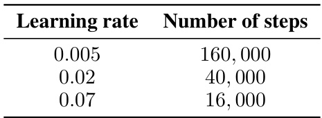
🔼 This table shows the hyperparameters used in the experiments presented in Figures 1a and 1b of the paper. It lists the learning rate used for gradient descent, the corresponding number of gradient descent steps performed, and the number of independent repetitions of the experiment for each learning rate. These hyperparameters were chosen to explore the impact of learning rate on training success and convergence, particularly in relation to the critical learning rate beyond which the training fails to converge (as described in Figure 1a).
read the caption
Table 1: Learning rate, number of steps, and number of repetitions for Figures 1a and 1b.
Full paper#


