↗ OpenReview ↗ NeurIPS Homepage ↗ Chat
TL;DR#
Estimating the nadir objective vector is crucial in multi-objective optimization, guiding the search and normalizing the objective space. However, current methods struggle with complex problems, failing to accurately estimate this vector for problems with irregular Pareto fronts. This limitation hinders the effectiveness of many optimization algorithms.
This research introduces BDNE, a boundary decomposition method that addresses these issues. BDNE scalarizes the problem into manageable subproblems, utilizing bilevel optimization to iteratively refine solutions and precisely estimate the nadir objective vector. The theoretical analysis shows BDNE’s effectiveness under mild conditions, and extensive experiments on diverse problems demonstrate its superior performance over existing methods, opening new possibilities for real-world applications and further research in multi-objective optimization.
Key Takeaways#
Why does it matter?#
This paper is important because it presents BDNE, a novel and robust method for estimating the nadir objective vector in multi-objective optimization problems. This is crucial because accurate nadir objective vector estimation is vital for many optimization algorithms and decision-making processes. BDNE’s theoretical guarantees and strong empirical performance make it a significant contribution to the field. The method opens new avenues for research into efficient and reliable multi-objective optimization techniques, particularly for complex problems with irregular Pareto fronts.
Visual Insights#

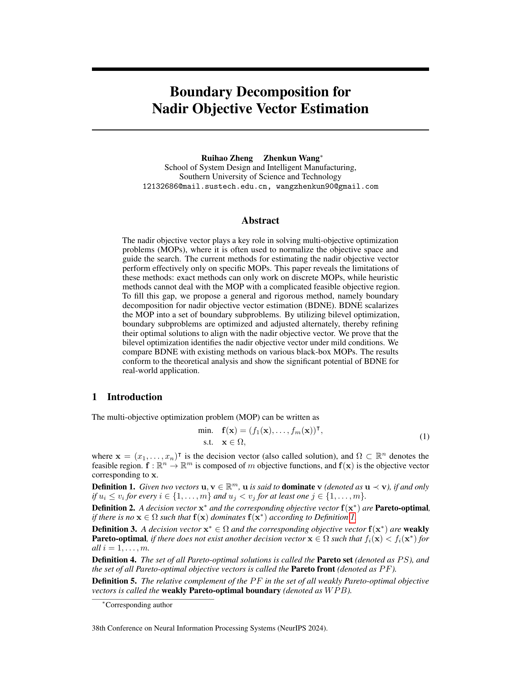
This figure illustrates the contour surfaces of boundary subproblems for different weight vectors. It shows how the shape of the contour surface changes depending on the weights assigned to each objective function. Specifically, it demonstrates that different weight vectors result in different optimal objective vectors, illustrating the impact of weight selection in the boundary decomposition method.

This table lists the symbols used in Section 3.3 of the paper and their corresponding descriptions. The symbols represent various parameters and variables used in the Boundary Decomposition for Nadir Objective Vector Estimation (BDNE) algorithm, including the maximum number of iterations for the CMA-ES procedure, the number of generated lower-level optimization problems (LLOPs), the population size of the multi-objective evolutionary algorithm (MOEA), the size of the elite archive, and boundary weight vectors.
In-depth insights#
Nadir Vector Estimation#
Nadir vector estimation is a crucial aspect of multi-objective optimization, aiming to identify the worst Pareto optimal solution. Accurate estimation is vital because it influences normalization techniques, search guidance within algorithms, and the overall understanding of the Pareto front. Traditional methods face limitations, particularly with complex problem structures or continuous objective spaces. Exact methods often struggle beyond discrete problems, while heuristics lack robustness and theoretical guarantees. Therefore, the development of a reliable, generalizable nadir vector estimation method remains an active area of research. The ideal approach would be mathematically rigorous, handle diverse problem landscapes, and provide practical tools for real-world applications. Future work in this area could focus on enhancing the efficiency of existing techniques, exploring novel methodologies, and investigating the impact of imprecise estimations on various multi-objective algorithms.
Boundary Decomposition#
Boundary decomposition, in the context of optimization problems, is a powerful technique for tackling complex, high-dimensional problems. It strategically breaks down a large problem into smaller, more manageable subproblems, each focusing on a specific region or aspect of the solution space. This decomposition is particularly effective when dealing with non-convex or irregular solution spaces, where traditional methods may struggle. The core of this approach lies in its ability to simplify the problem’s structure, making it more amenable to analysis and solution. This is achieved by defining boundaries that partition the solution space, allowing for localized optimization within each region. The boundaries themselves may be defined based on various criteria, such as geometric properties of the solution space or characteristics of the objective functions. A key advantage of this method is its potential for parallelization, as the subproblems can be solved independently. Once solved, the results from the subproblems can be combined or compared, providing a comprehensive solution to the original problem. However, careful consideration must be given to how the boundaries are defined and how the results from the subproblems are aggregated, ensuring a holistic solution. Furthermore, the effectiveness of boundary decomposition is highly dependent on the nature of the problem and the choice of decomposition strategy. For some problems, the benefits of decomposition may outweigh the costs of dividing and combining the subproblems, while for others, it might be less advantageous.
Bilevel Optimization#
Bilevel optimization, in the context of nadir objective vector estimation, presents a powerful framework for tackling complex multi-objective optimization problems. The core idea revolves around a hierarchical optimization structure. The upper level focuses on strategically adjusting parameters, such as boundary weight vectors, to effectively guide the search process toward the nadir vector. This adjustment is informed by the lower level, which optimizes a series of boundary subproblems. Each subproblem scalarizes the original multi-objective problem. This iterative interplay between the upper and lower levels ensures that boundary solutions are progressively refined, converging towards the nadir objective vector. The theoretical guarantees BDNE offers stem from the careful design of the boundary subproblems and rigorous analysis of the bilevel optimization process. This bilevel approach proves to be particularly useful when dealing with problems having irregular Pareto fronts or complex feasible regions, which often pose significant challenges for traditional heuristic methods. The approach effectively balances the need for both exploration and exploitation, making it a versatile solution for a broad range of multi-objective optimization problems. The use of bilevel optimization is key to BDNE’s ability to handle black-box problems and achieve significant improvement over traditional methods.
BDNE Algorithm#
The BDNE (Boundary Decomposition for Nadir Objective Vector Estimation) algorithm presents a novel approach to a long-standing challenge in multi-objective optimization: accurately estimating the nadir objective vector. BDNE’s core innovation lies in its scalarization technique, which decomposes the multi-objective problem into a series of boundary subproblems. This decomposition, coupled with a bilevel optimization strategy, allows for the iterative refinement of solutions, ultimately converging towards the nadir objective vector. A key strength of BDNE is its theoretical rigor, backed by proofs demonstrating its effectiveness under relatively mild conditions. Unlike heuristic methods which often struggle with complex feasible regions, BDNE offers a more robust and generalizable solution. The algorithm’s performance is further enhanced through the incorporation of normalization and a user-defined trade-off parameter, allowing for a degree of customization to suit specific problem contexts and decision-maker preferences. While computationally more expensive than heuristic methods, BDNE’s theoretical guarantees and superior performance on a wide range of benchmark problems, especially those with irregular Pareto fronts, highlight its potential as a significant advancement in multi-objective optimization.
Future Research#
Future research directions stemming from this boundary decomposition for nadir objective vector estimation (BDNE) method could explore several promising avenues. Improving BDNE’s efficiency for high-dimensional problems is crucial, perhaps through the development of more sophisticated optimization algorithms or dimensionality reduction techniques. Incorporating user preferences more directly into the BDNE framework could enhance its practical applicability by allowing decision-makers to guide the search towards desirable solutions. The current method assumes a certain level of user-defined tolerance for trade-offs; more research on adaptively determining this tolerance could lead to a more robust and effective approach. Finally, further investigation into the theoretical properties of BDNE and its relationship to other multi-objective optimization techniques could provide valuable insights and potentially lead to novel algorithms. Extending BDNE to handle stochastic or dynamic MOPs would significantly broaden its range of applicability and address a critical need in many real-world applications.
More visual insights#
More on figures

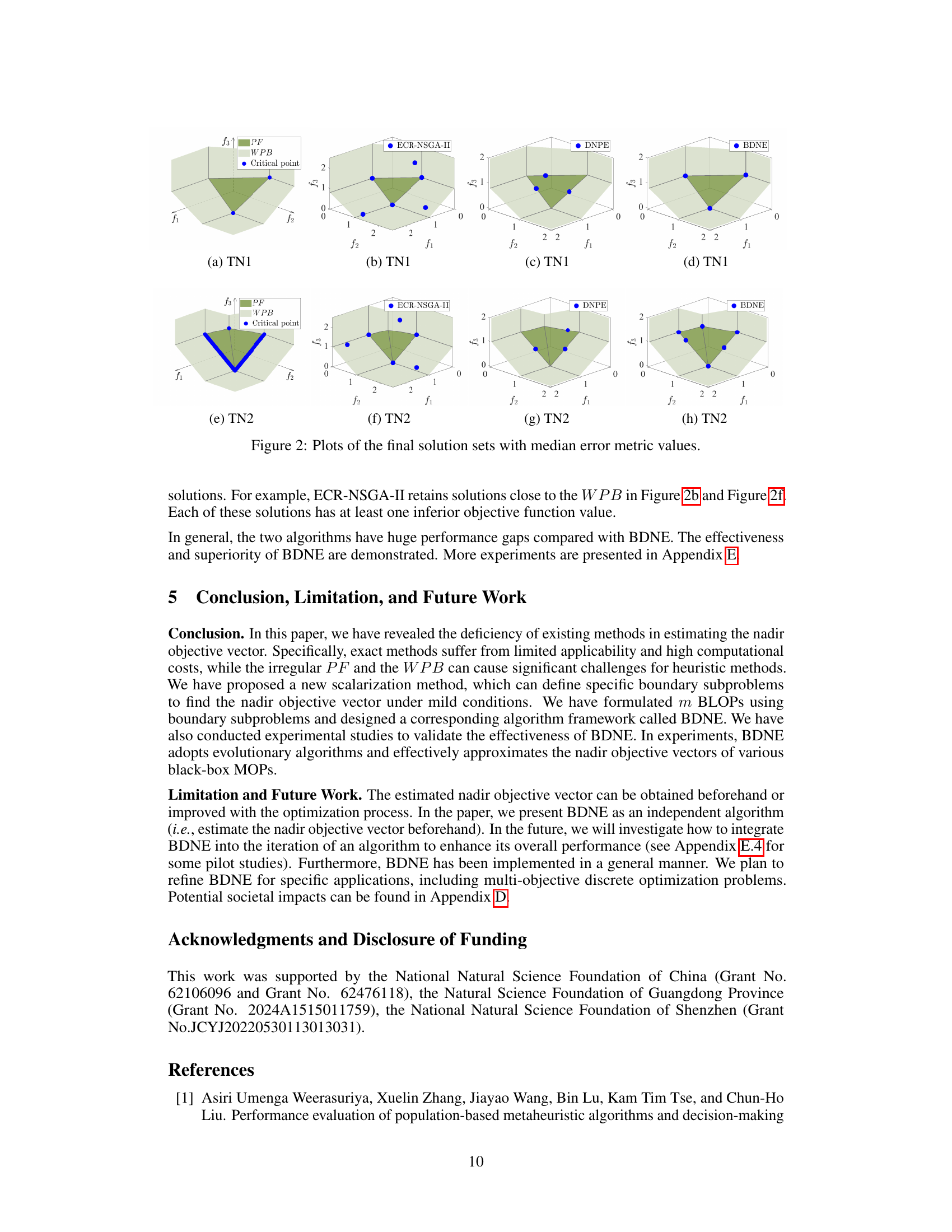
This figure shows the final solution sets obtained by three different algorithms (ECR-NSGA-II, DNPE, and BDNE) for two different test problems (TN1 and TN2), each with three objectives. The plots visualize the distribution of the solutions in the objective space, highlighting the performance of each algorithm in finding the Pareto front (PF). The plots illustrate the shortcomings of ECR-NSGA-II and DNPE in accurately approximating the critical points and nadir objective vector, particularly in the case of TN2, which has a more complex feasible region. In contrast, BDNE effectively locates the critical points and approximates the nadir objective vector more accurately in both scenarios. The median error metric values are also indicated for each algorithm and problem.
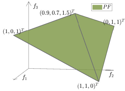
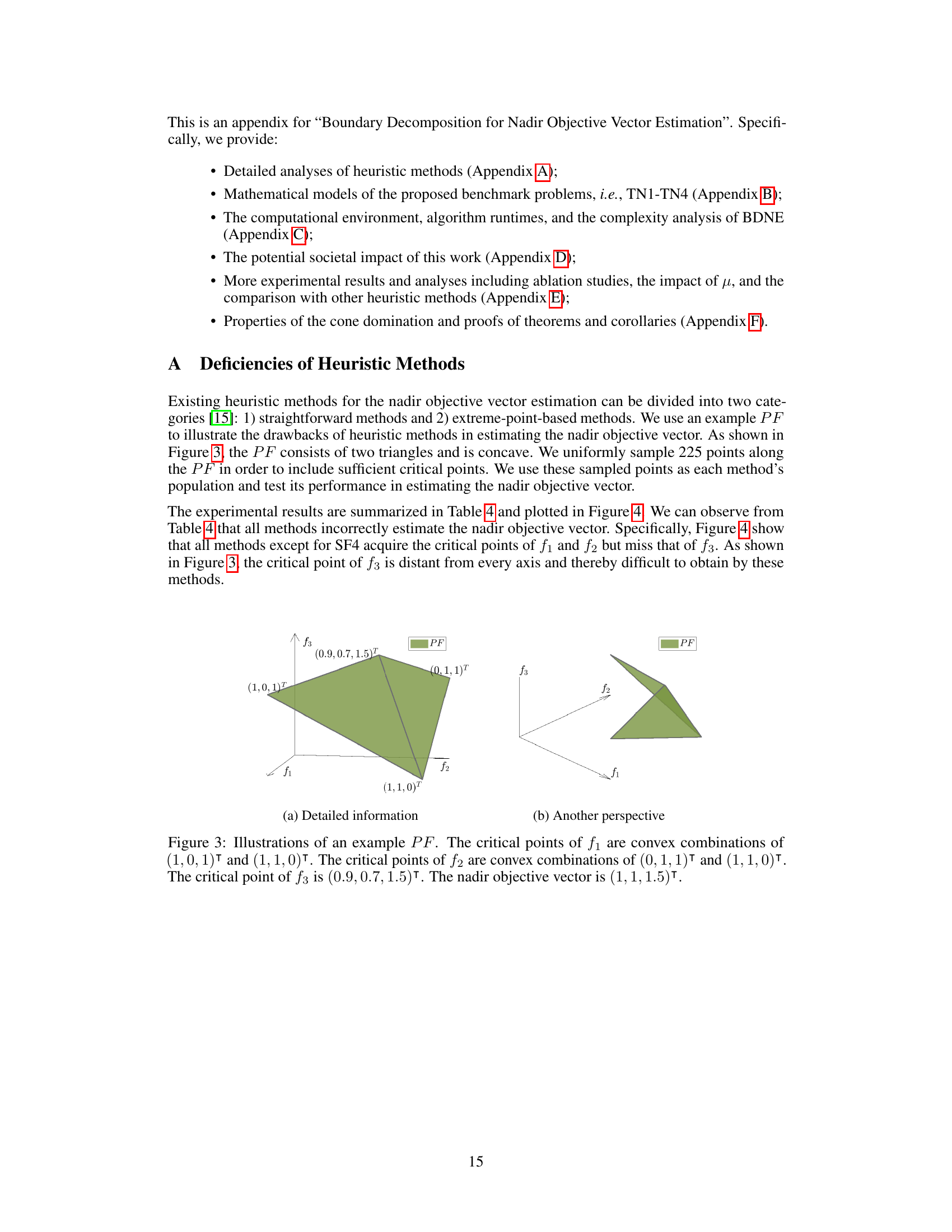
This figure shows an example of a Pareto front (PF) with two triangles, illustrating the concept of critical points. The critical points, indicated by their coordinates, represent Pareto optimal solutions that have the worst value in each objective function. The figure also points out the nadir objective vector which consists of the upper bounds of the Pareto front.
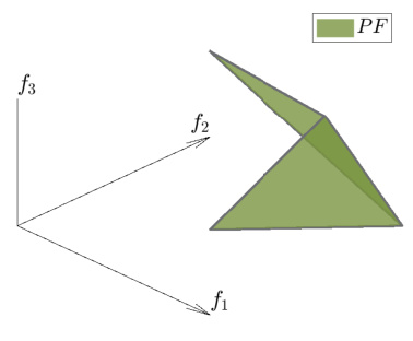
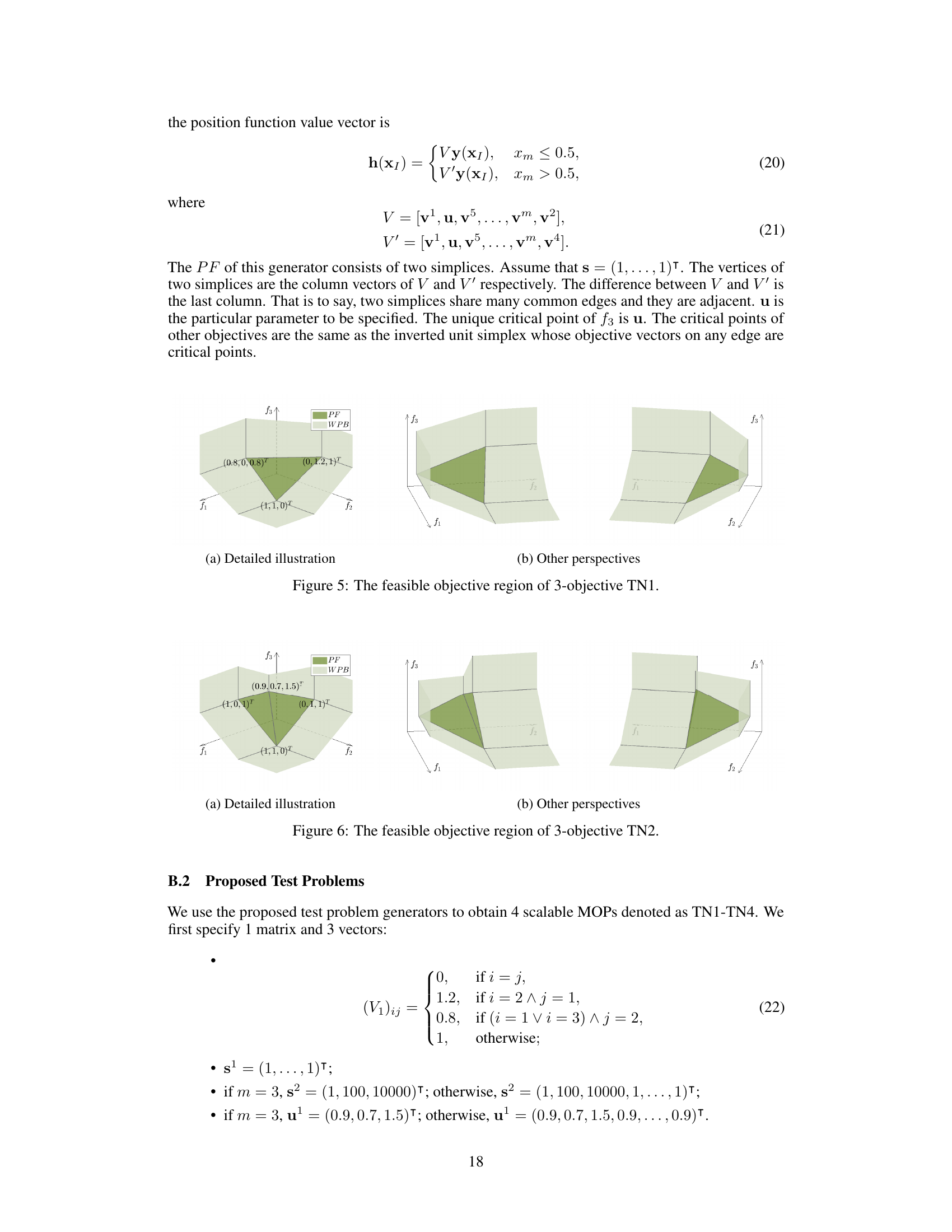
The figure shows the feasible objective region of a 3-objective test problem (TN2). The Pareto front (PF) is shown in green, and has a concave shape, consisting of two adjacent simplices. The figure illustrates the complexity of the feasible region, emphasizing the challenges in accurately estimating the nadir objective vector, which is a critical point for multi-objective optimization. The concave shape makes it difficult for simpler heuristic methods to accurately find the nadir objective vector.
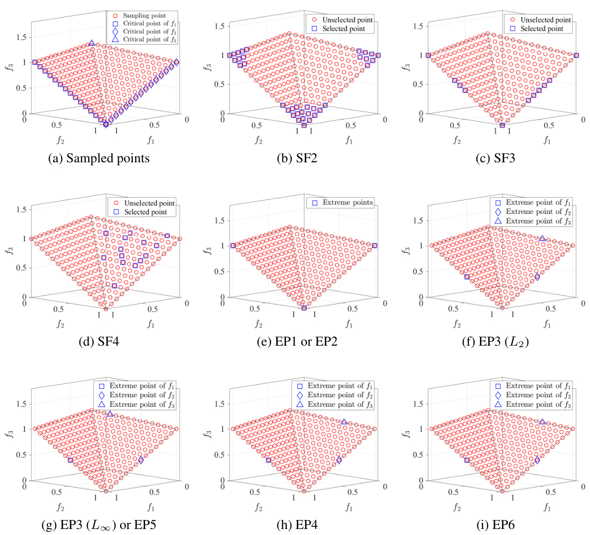
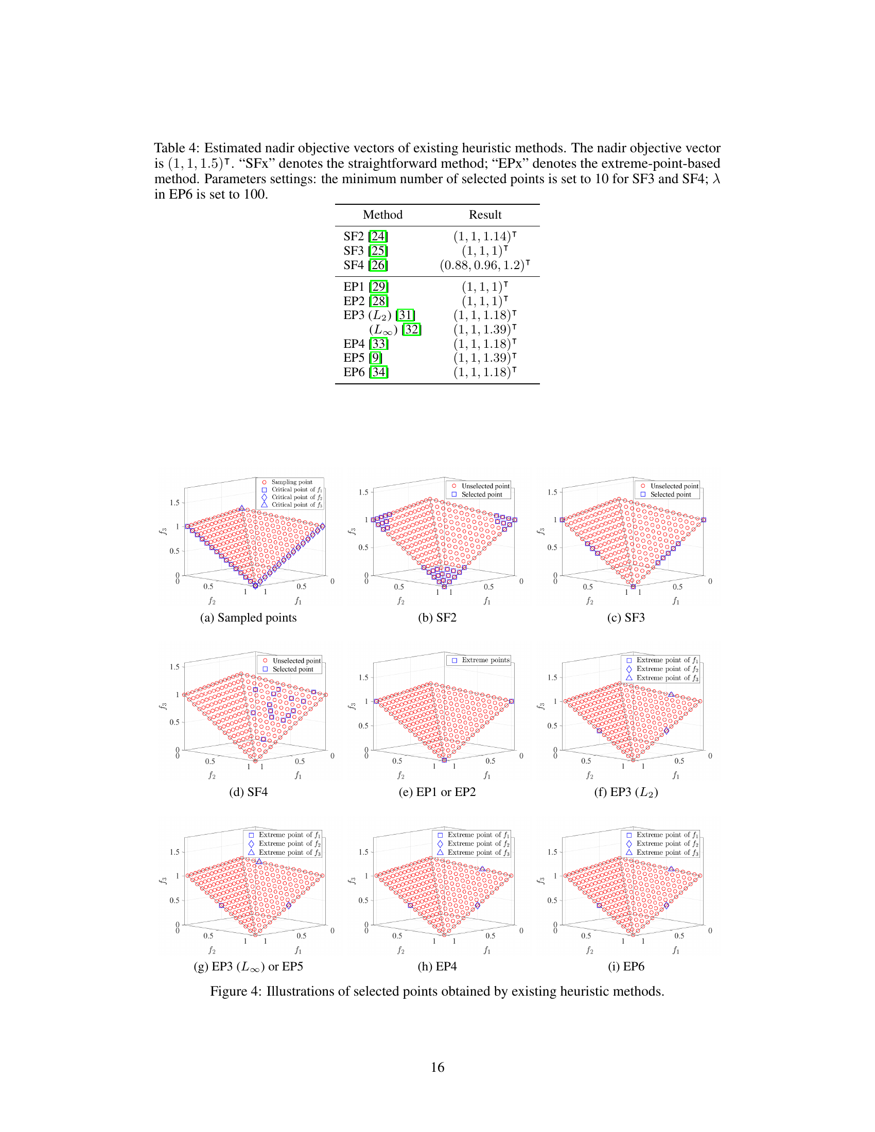
This figure displays visualizations of the points selected by various heuristic methods for nadir objective vector estimation. The different methods (SF2, SF3, SF4, EP1/EP2, EP3 (L∞)/EP5, EP3 (L2), EP4, EP6) are shown selecting different points along the Pareto front (PF) and weakly Pareto-optimal boundary (WPB). The plots illustrate the differences in point selection behavior across various methods.

The figure shows the feasible objective region of the 3-objective TN1 problem. The detailed illustration (a) shows the Pareto front (PF) and weakly Pareto boundary (WPB), highlighting the critical points that are the vertices of the two simplices forming the PF. The other perspectives (b) show the same feasible region from different angles. The PF is formed by two simplices that share an edge (where the critical point of f3 lies). The critical points for f1 and f2 are the vertices of the simplices. This figure illustrates the relationship between the Pareto front and the critical points of the TN1 problem.

The figure shows the feasible objective region and Pareto front (PF) of a 3-objective TN2 problem. The PF is shown in olive green, and the weakly Pareto-optimal boundary (WPB) is in light green. The figure highlights the concave shape of the Pareto front and illustrates the location of the critical points for each objective function, showcasing a complex geometry that poses challenges to many existing nadir objective vector estimation methods. The concave shape of the PF, in particular, makes it difficult for heuristic methods to accurately identify the nadir objective vector.
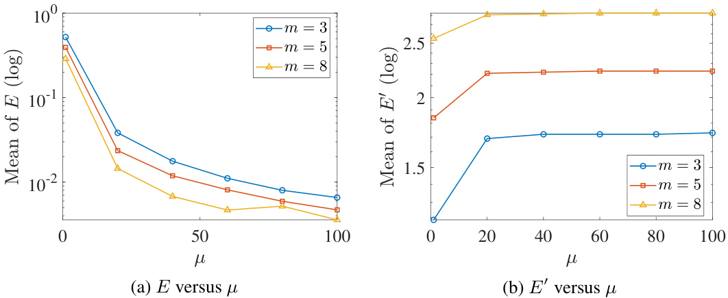
The plots show the mean of the error metric (E) and the mean of the distance between the estimated nadir objective vector and the ideal objective vector (E’) for different values of μ (1, 20, 40, 60, 80, and 100) on the mDTLZ2 problem. The results illustrate the impact of the parameter μ on the accuracy of nadir objective vector estimation and suggest a trade-off between accuracy and the decision-maker’s preference for solutions. A smaller μ leads to a smaller set of preferred solutions and increases the distance from the exact nadir objective vector while increasing the accuracy.

This figure shows the impact of changing the maximum number of iterations (Tu) in the upper-level optimization of the BDNE algorithm on the TN4 problem. It contains two sub-figures: (a) shows the mean error (E) against Tu for different numbers of objectives (m=3, 5, 8), and (b) shows the mean runtime against Tu for the same objective counts. The results demonstrate a generally decreasing error with increasing Tu, indicating improved accuracy with more iterations, although with some fluctuations due to the stochastic nature of the lower-level optimization algorithm. The runtime increases linearly with Tu.
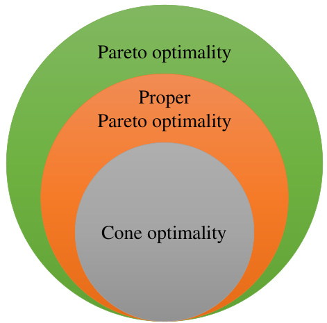
This figure is a Venn diagram that visually represents the relationships between three types of optimality: Pareto optimality, proper Pareto optimality, and cone optimality. It shows that cone optimality is a subset of proper Pareto optimality, which in turn is a subset of Pareto optimality. This illustrates the hierarchical nature of these optimality concepts, with cone optimality being the most restrictive and Pareto optimality the least restrictive.
More on tables
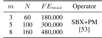
This table shows the general settings used for the three algorithms compared in the paper: ECR-NSGA-II, DNPE, and BDNE. The settings include the number of objectives (m), the population size (N), the maximum number of function evaluations (FEmax), and the genetic operators used (SBX+PM). These parameters control the computational budget and the search strategy employed by each algorithm.
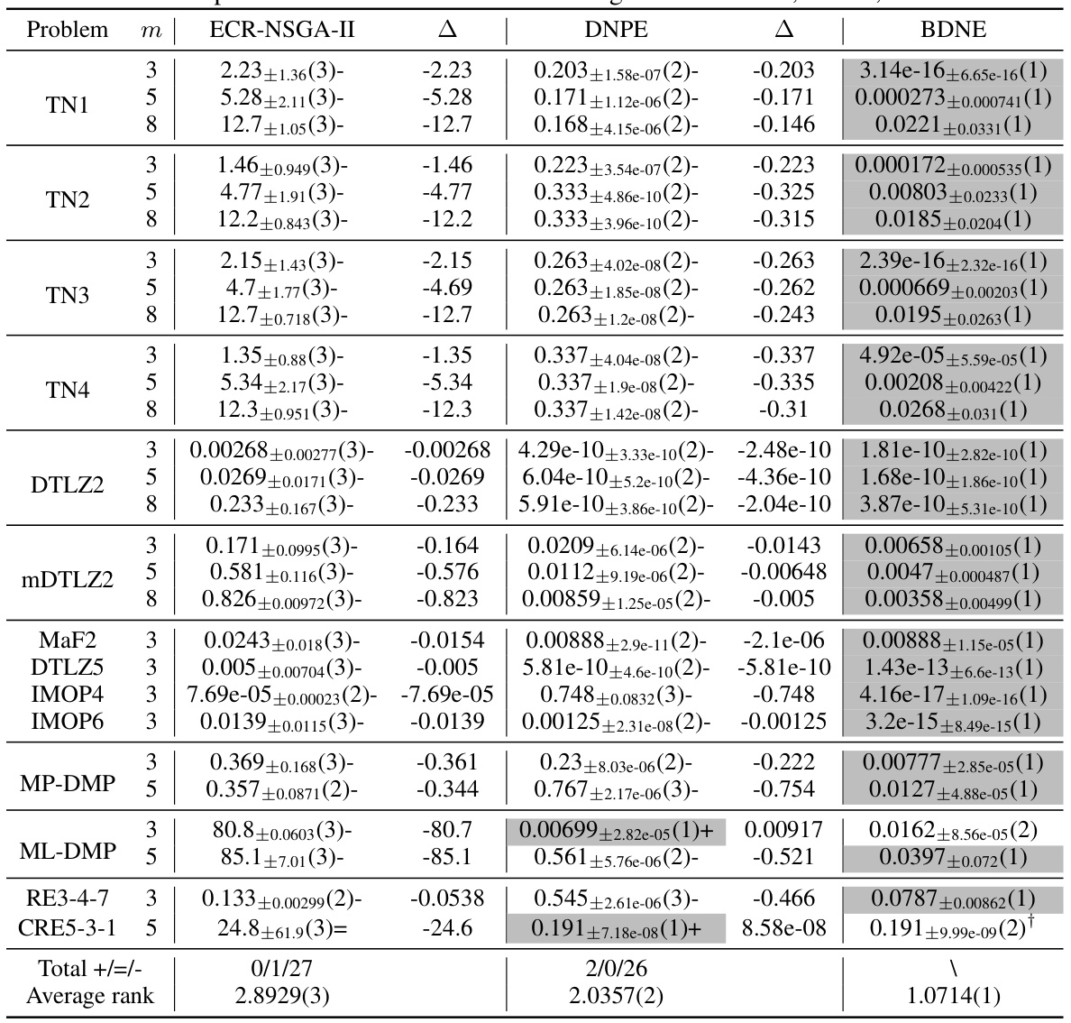
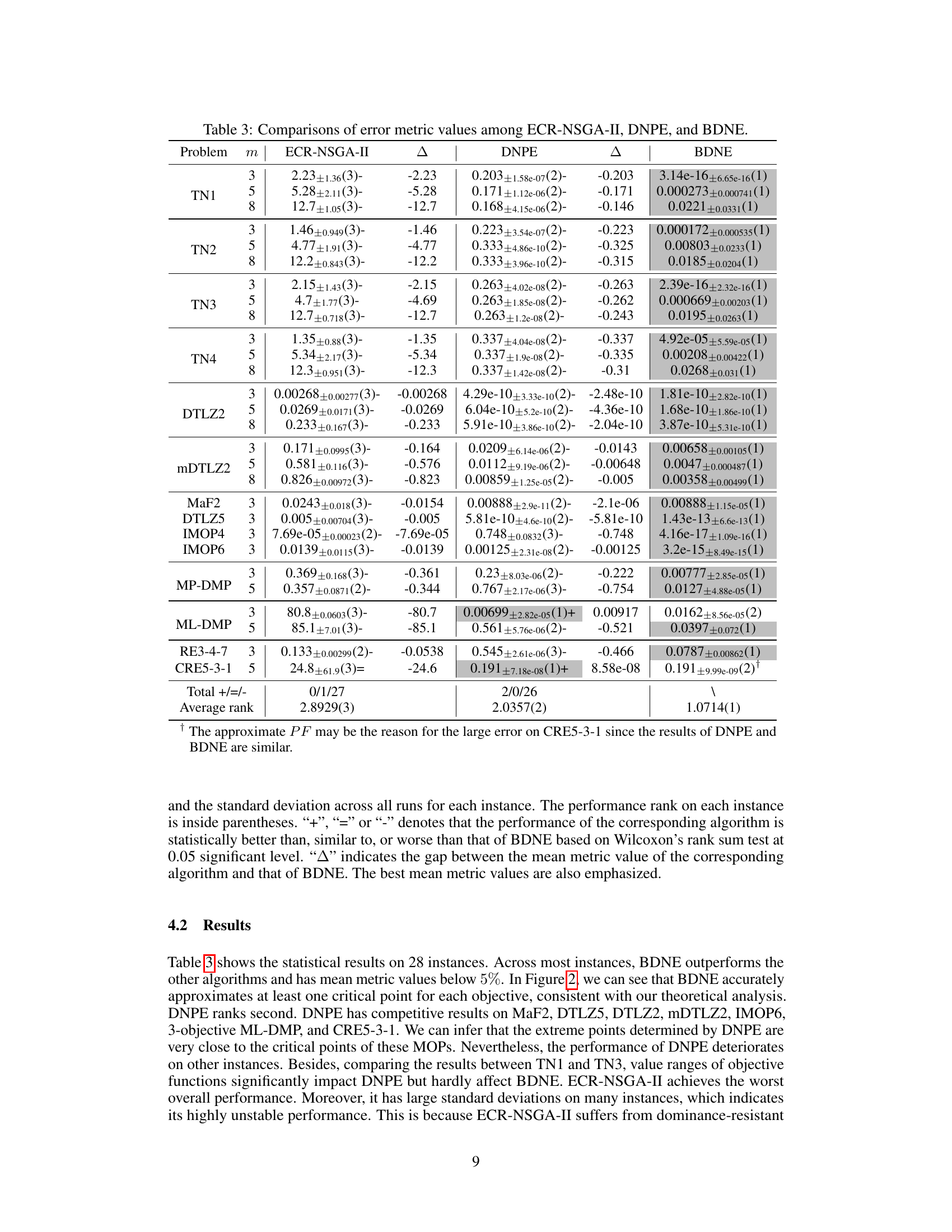
This table presents a comparison of the error metric values obtained by three different algorithms: ECR-NSGA-II, DNPE, and BDNE. The error metric quantifies the accuracy of each algorithm in estimating the nadir objective vector. The table shows results for various multi-objective optimization problems (MOPs), categorized by problem name, number of objectives (m), and including the mean error metric and its standard deviation across multiple runs. The best results for each instance are highlighted, and statistical significance is indicated using symbols (+, =, -) based on Wilcoxon’s rank sum test to show if there is statistically significant difference between the performances of each algorithm in each problem instance.
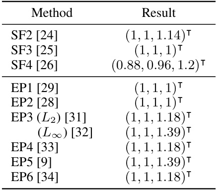
This table presents the estimated nadir objective vectors obtained using various heuristic methods (straightforward and extreme-point based). The results are compared against the true nadir objective vector (1, 1, 1.5). The table highlights the limitations of these methods in accurately estimating the nadir objective vector, especially for complex Pareto fronts. Parameters used in each method are also specified.

This table presents the parameter settings used to generate four scalable multi-objective optimization problems (TN1-TN4). It includes the problem generator used (Generator 1 or 2), and the specific parameter values for each problem, including the scaling vector ’s’ and the vertices of the PF ‘V’ or the critical point ‘u’. The nadir objective vector for each problem is also provided.
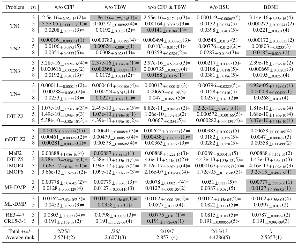
This table presents a comparison of the error metric values obtained by three different algorithms: ECR-NSGA-II, DNPE, and BDNE, across various test problems. The problems vary in the number of objectives (3, 5, or 8) and their characteristics. The error metric quantifies how well each algorithm estimates the nadir objective vector. Smaller values indicate better performance. The table also includes the mean error and standard deviation for each algorithm on each problem. Additionally, statistical significance tests are performed to compare the performance of the algorithms and the results are shown using symbols (+, =, -). The best mean error values are highlighted.
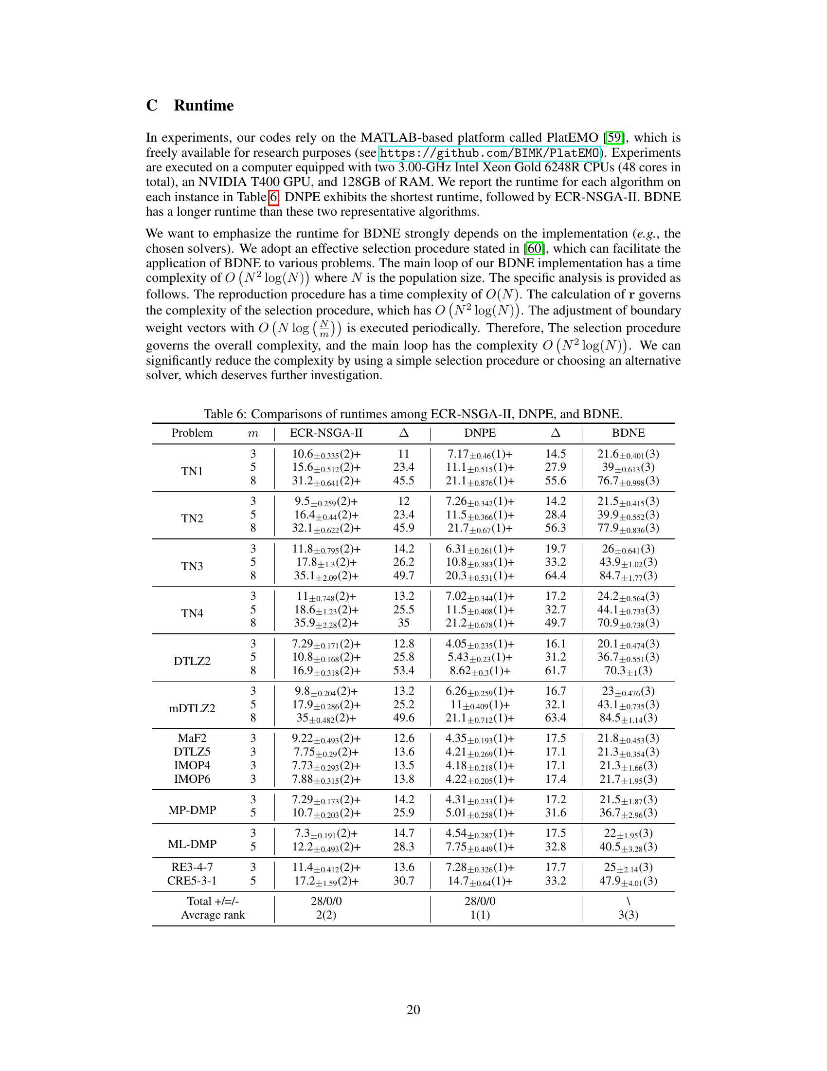
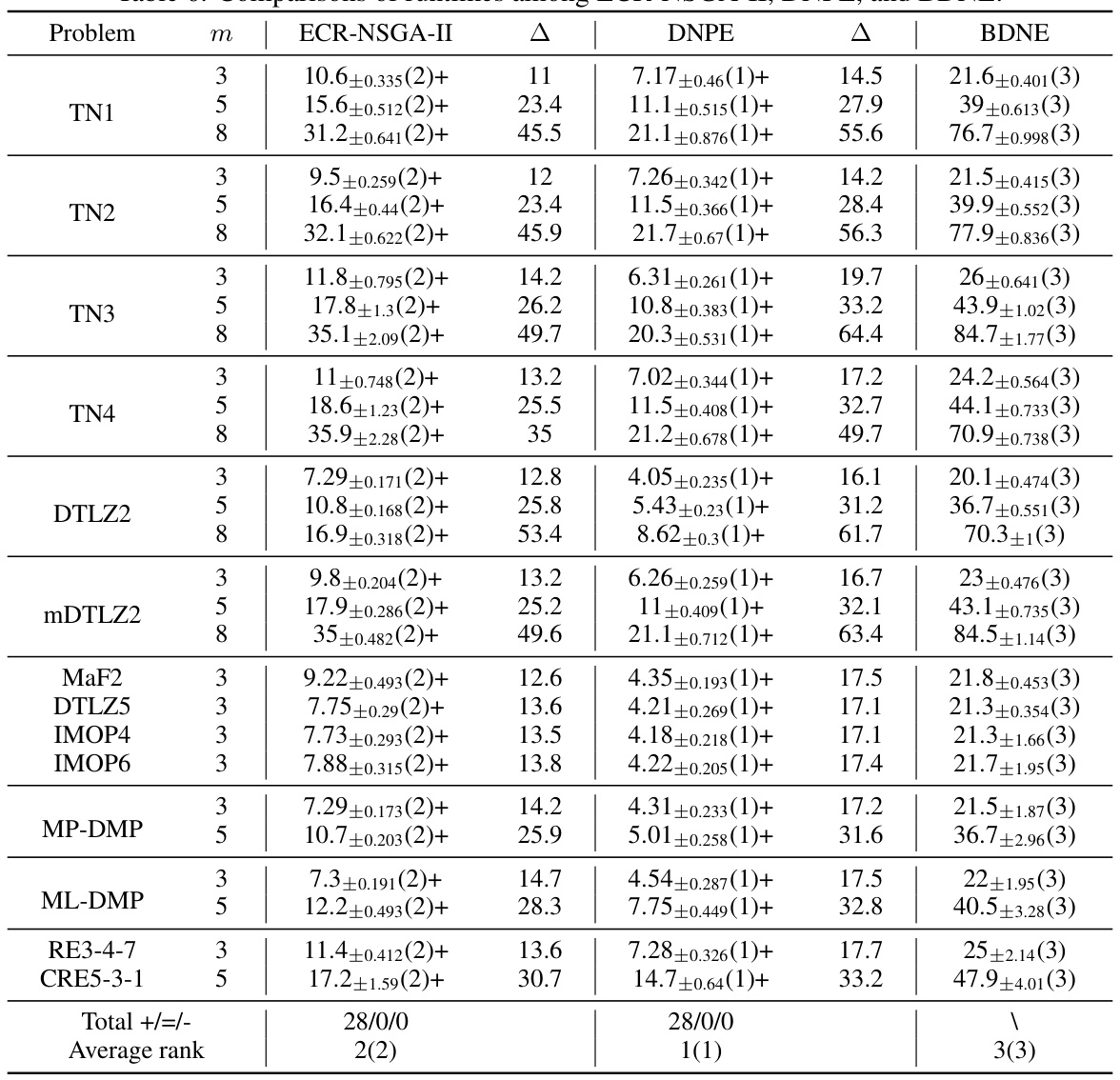
This table presents the results of comparing three algorithms (ECR-NSGA-II, DNPE, and BDNE) across various multi-objective optimization problems. For each problem, the table shows the mean error metric and its standard deviation across 30 independent runs. The ‘Δ’ column indicates the difference between the mean error of each method and that of BDNE. The numbers in parentheses indicate the statistical rank of each algorithm on that problem instance, with lower ranks indicating better performance. The plus, equals, and minus signs denote whether a method’s performance is statistically significantly better than, similar to, or worse than BDNE, respectively.

This table summarizes the performance comparison of BDNE against other heuristic methods for nadir objective vector estimation across various test problems. It shows the total number of instances where each method outperformed BDNE, and the average ranks of all methods across the instances.

This table presents the results of comparing three different algorithms (ECR-NSGA-II, DNPE, and BDNE) for estimating the nadir objective vector. The comparison is done across various test problems (TN1-TN4, DTLZ2, mDTLZ2, MaF2, DTLZ5, MP-DMP, ML-DMP, RE3-4-7, and CRE5-3-1) with different numbers of objectives (3, 5, and 8). For each problem and number of objectives, the table shows the mean error metric values and standard deviations for each algorithm. The error metric is calculated based on the estimated and the actual nadir objective vector. Parentheses indicate the rank of the algorithm for each instance based on the error metrics.

This table presents the comparison results of three algorithms (ECR-NSGA-II, DNPE, and BDNE) using an error metric on 28 benchmark problems. Each problem is tested with varying numbers of objectives (3, 5, and 8). The results are presented as mean ± standard deviation and the rank of the algorithms on each problem. The symbols (+, =, -) indicate whether the performance of the corresponding algorithm is statistically better than, similar to, or worse than that of BDNE based on Wilcoxon’s rank-sum test at a 0.05 significance level. Δ represents the gap between the mean metric value of the corresponding algorithm and that of BDNE. The best mean metric values are emphasized.

This table summarizes the overall performance comparison of three multi-objective optimization algorithms (ECR-NSGA-II, DNPE, and BDNE) across different test problem suites (MaF, mDTLZ, and IMOP). The results are presented in terms of the number of instances where each algorithm outperforms the others, indicating the relative strengths and weaknesses of each approach across diverse problem characteristics.

This table presents a comparison of the performance of three different algorithms (ECR-NSGA-II, DNPE, and BDNE) for estimating the nadir objective vector on 28 benchmark problems. The performance is measured using an error metric, and the table shows the mean error and standard deviation across multiple runs for each problem and algorithm. The symbol (△) shows the gap between the mean metric value of the corresponding algorithm and that of BDNE. The best mean metric values are also emphasized.
Full paper#
