TL;DR#
Predicting the behavior of molecules and materials requires computationally expensive simulations. Machine-learned interatomic potentials (MLIPs) offer a faster alternative by learning from high-quality data. However, current MLIPs using spherical tensors are computationally expensive for high-rank tensors. Existing Cartesian tensor-based methods lack flexibility and expressive power.
This research introduces a novel approach using higher-rank irreducible Cartesian tensors within message-passing neural networks. The researchers demonstrate that this method provides comparable or superior performance to state-of-the-art spherical and Cartesian models, offering a more flexible and efficient way to represent atomic systems. The method’s equivariance and traceless properties are mathematically proven, enhancing its reliability. Experiments show improved results across several benchmark datasets, indicating the method’s effectiveness.
Key Takeaways#
Why does it matter?#
This paper is crucial for researchers in materials science and chemistry. It significantly advances the field of machine-learned interatomic potentials by introducing a novel and efficient method using irreducible Cartesian tensors. This offers a significant improvement over existing methods, paving the way for more accurate and computationally cheaper simulations of complex systems.
Visual Insights#

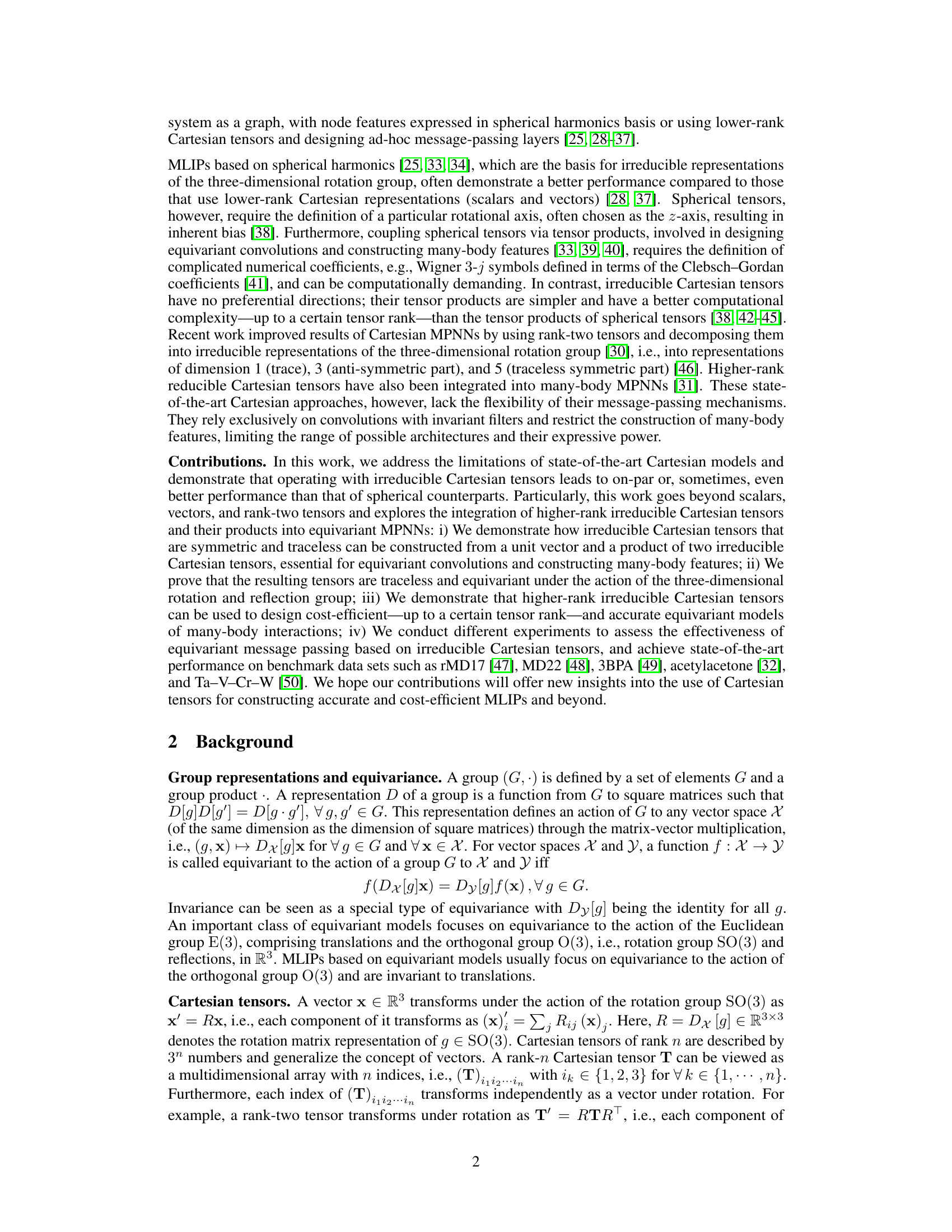
🔼 This figure schematically illustrates the construction of irreducible Cartesian tensors and their products. (a) shows how to build a rank-l irreducible Cartesian tensor from a unit vector. (b) demonstrates the tensor product of two irreducible Cartesian tensors, resulting in a new tensor of rank l3 which can be even or odd depending on l₁ + l₂ - l3. The transparent boxes highlight the linearly dependent elements of the symmetric and traceless tensors.
read the caption
Figure 1: Schematic illustration of (a) the construction of an irreducible Cartesian tensor for a local atomic environment and (b) the tensor product of two irreducible Cartesian tensors of rank l₁ and l₂. The construction of an irreducible Cartesian tensor from a unit vector î is defined in Eq. (1). In this work, we use tensors with the same rank n and weight l, i.e., n = l, avoiding the need for embedding tensors with l < n in a higher-dimensional tensor space. Therefore, we use l to identify the rank and the weight of an irreducible Cartesian tensor. The tensor product is defined in Eqs. (2) and (3), resulting in a new tensor Tl3 = (Tl₁ Cart T12) 13 of rank l3 = {|l₁ - l₂|,··· ,l₁ + l₂}. Transparent boxes denote the linearly dependent elements of symmetric and traceless tensors. The tensor product can be even or odd, defined by l₁ + l₂ - l3.
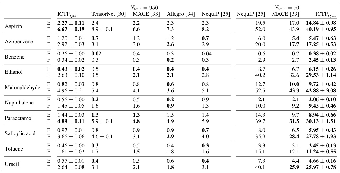
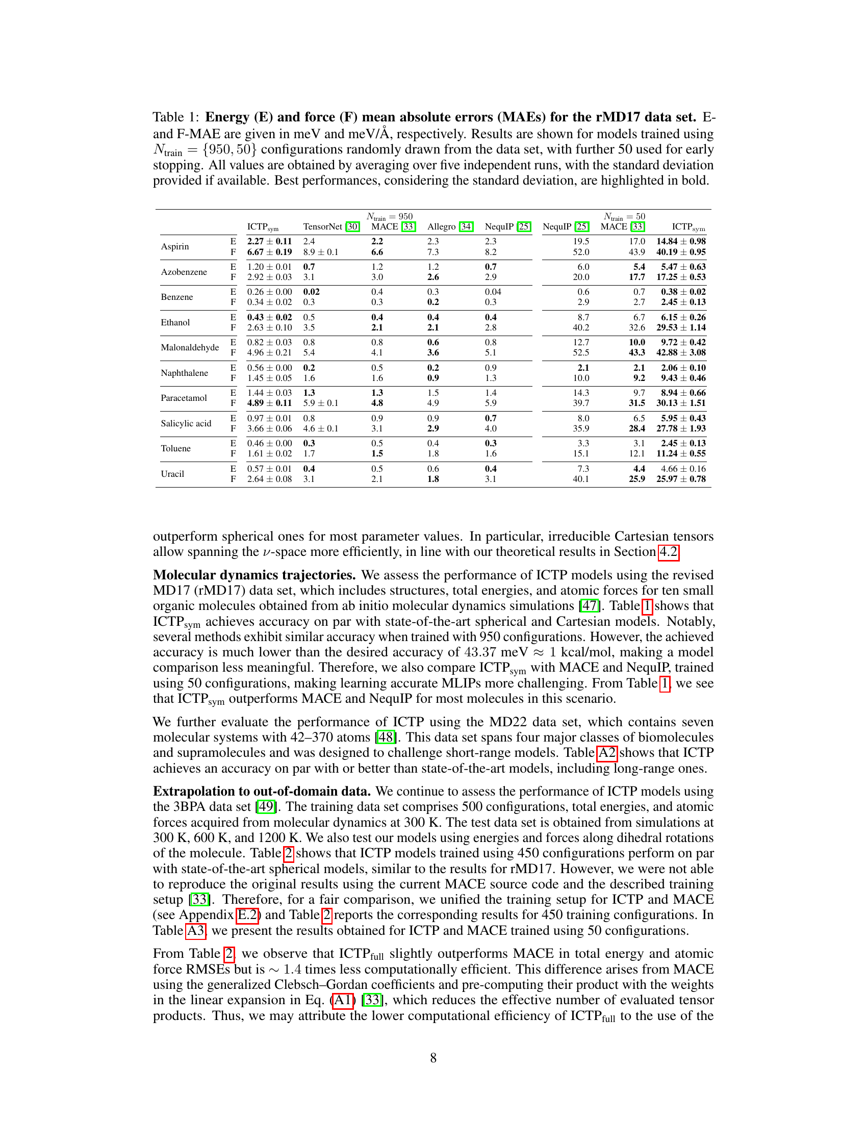
🔼 This table presents the mean absolute errors (MAE) in total energies (E) and atomic forces (F) for models trained on the rMD17 dataset. The models were trained with either 950 or 50 configurations, and the results are averages of five independent runs. The best-performing models, taking into account the standard deviation, are shown in bold. The MAEs are given in meV for energy and meV/Å for force.
read the caption
Table 1: Energy (E) and force (F) mean absolute errors (MAEs) for the rMD17 data set. E-and F-MAE are given in meV and meV/Å, respectively. Results are shown for models trained using Ntrain = {950, 50} configurations randomly drawn from the data set, with further 50 used for early stopping. All values are obtained by averaging over five independent runs, with the standard deviation provided if available. Best performances, considering the standard deviation, are highlighted in bold.
In-depth insights#
Equivariant MPNNs#
Equivariant message-passing neural networks (MPNNs) represent a significant advancement in geometric deep learning, particularly within the context of atomistic simulations. Equivariance is a crucial property, ensuring that the model’s output transforms predictably under certain group actions (e.g., rotations, translations, reflections) applied to the input data. This inductive bias greatly improves efficiency and accuracy by reducing the amount of training data needed and enhancing generalizability. In the field of atomistic simulations, equivariant MPNNs leverage this to encode the crucial directional information inherent in molecular structures, leading to more physically meaningful representations. Spherical harmonics have been popularly used, but Cartesian tensors offer a compelling alternative with potentially improved computational efficiency and flexibility, especially for higher-rank tensors, as explored in the provided research. The choice between these representations involves a trade-off between computational cost and representational power, highlighting an active area of research in developing efficient and accurate equivariant MPNNs for complex systems.
Cartesian tensors#
The concept of Cartesian tensors, as described in the paper, offers a compelling alternative to spherical tensors for representing atomic systems in machine-learned interatomic potentials. Unlike spherical tensors, which necessitate defining a specific rotational axis and complex numerical coefficients (Wigner 3j symbols) when computing tensor products, Cartesian tensors inherently lack this directional bias and their products simplify calculations. The paper particularly emphasizes higher-rank irreducible Cartesian tensors, proving their equivariance and traceless property within message-passing neural networks. This approach enhances flexibility by overcoming limitations in current Cartesian models, where message-passing mechanisms were restricted. The key advantage lies in the computationally efficient construction of many-body features due to the simpler nature of the tensor products. The integration of irreducible Cartesian tensors enables on-par or superior performance in various benchmark datasets, demonstrating the potential for more efficient and accurate atomistic simulations.
Tensor products#
The concept of tensor products is crucial for constructing equivariant neural networks, particularly in the context of message-passing models for atomistic simulations. The paper explores the use of higher-rank irreducible Cartesian tensors, which offer advantages over spherical tensors in terms of computational efficiency and flexibility. Irreducible Cartesian tensors avoid the need for defining a preferential axis, simplifying calculations. However, the process of constructing tensor products is computationally demanding, even with Cartesian tensors, especially as the rank increases. The authors demonstrate how irreducible Cartesian tensor products can be constructed efficiently to create higher-order features for many-body interactions, proving both equivariance and the traceless property of the resulting layers. This addresses a key limitation in existing Cartesian models by enabling the efficient construction of more expressive architectures. The computational cost-effectiveness is particularly relevant for high-rank tensors where methods using spherical tensors become significantly more expensive. Ultimately, these advancements improve the accuracy and scalability of machine-learned interatomic potentials.
Computational cost#
The research paper analyzes computational costs associated with different methods for constructing machine-learned interatomic potentials. Spherical harmonics-based models, while often exhibiting superior performance, incur high costs due to complicated numerical coefficients and tensor products requiring Clebsch-Gordan coefficients. In contrast, Cartesian tensor-based models offer a promising alternative but have lacked flexibility. The study introduces higher-rank irreducible Cartesian tensors which offer a potential for significant cost reduction in specific scenarios, mainly for lower tensor ranks. While the irreducible Cartesian tensor product avoids the expensive Clebsch-Gordan coefficient calculation, it’s noted that for very high tensor ranks, spherical approaches may remain more computationally efficient. The paper highlights a trade-off between computational cost and model expressiveness, emphasizing that choosing the optimal representation depends on the balance between accuracy requirements and computational resources.
Future work#
Future research directions stemming from this work could explore several promising avenues. Extending the framework to handle more complex chemical systems such as those involving long-range interactions or diverse bonding environments is a crucial next step. Investigating the application of irreducible Cartesian tensors to other graph-based machine learning tasks beyond atomistic simulations would also broaden the impact. This could involve exploring different message-passing schemes or combining irreducible Cartesian tensors with other advanced neural network architectures to improve efficiency and accuracy. Furthermore, a more thorough theoretical analysis of the computational complexity of the proposed methods, potentially identifying approximations that can reduce runtime without sacrificing accuracy, is needed. Finally, systematic comparisons with other state-of-the-art methods on a wider range of benchmark datasets would strengthen the conclusions and demonstrate the robustness of the approach.
More visual insights#
More on figures

🔼 This figure compares the inference time and GPU memory consumption of Irreducible Cartesian Tensor Potentials (ICTP) and MACE models as a function of tensor rank (L) and correlation order (v) for the 3BPA dataset. It demonstrates the scaling behavior of both models with increasing tensor rank and correlation order, highlighting the computational advantages of ICTP, particularly for higher-order correlations. The figure also emphasizes the memory limitations of the MACE approach when working with higher-order tensors due to the computationally expensive Clebsch-Gordan coefficients.
read the caption
Figure 2: Inference times and memory consumption as a function of the tensor rank L (a)-(b) and the correlation order v (c)-(d). All results are obtained for the 3BPA data set and lmax = L. We used eight feature channels to allow experiments with larger v values. MACE models use intermediate tensors with l > lmax for their product basis, which we fixed to l = lmax. Otherwise, pre-computing generalized Clebsch-Gordan coefficients for v > 4 would require more than 2 TB of RAM. For ICTP, we used the full product basis to compute the same number of v-fold tensor products as in MACE.

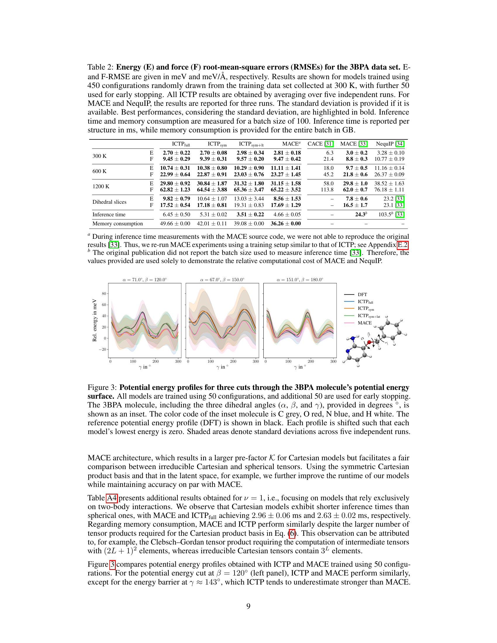
🔼 This figure compares the potential energy profiles of different models on the 3BPA molecule across three dihedral angles. The models were trained with limited data (50 configurations + 50 for early stopping) to show their generalization capabilities. The shaded areas show the standard deviation across multiple runs. The DFT curve serves as the ground truth.
read the caption
Figure 3: Potential energy profiles for three cuts through the 3BPA molecule's potential energy surface. All models are trained using 50 configurations, and additional 50 are used for early stopping. The 3BPA molecule, including the three dihedral angles (α, β, and γ), provided in degrees °, is shown as an inset. The color code of the inset molecule is C grey, O red, N blue, and H white. The reference potential energy profile (DFT) is shown in black. Each profile is shifted such that each model's lowest energy is zero. Shaded areas denote standard deviations across five independent runs.

🔼 The figure displays potential energy profiles for three different dihedral angle combinations of the 3BPA molecule. The profiles generated by different machine learning models (ICTPfull, ICTPsym, ICTPsym+lat, and MACE) are compared to Density Functional Theory (DFT) calculations. The shaded areas represent standard deviations. The inset shows the 3BPA molecule with its three dihedral angles labelled.
read the caption
Figure 3: Potential energy profiles for three cuts through the 3BPA molecule's potential energy surface. All models are trained using 50 configurations, and additional 50 are used for early stopping. The 3BPA molecule, including the three dihedral angles (α, β, and γ), provided in degrees °, is shown as an inset. The color code of the inset molecule is C grey, O red, N blue, and H white. The reference potential energy profile (DFT) is shown in black. Each profile is shifted such that each model's lowest energy is zero. Shaded areas denote standard deviations across five independent runs.
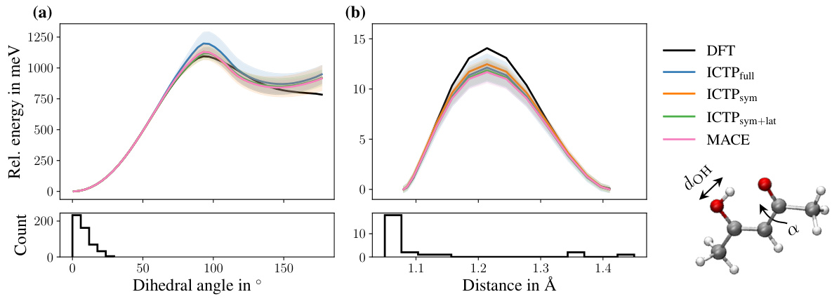
🔼 This figure compares the potential energy profiles obtained with different models (ICTPfull, ICTPsym, ICTPsym+lat, and MACE) for the 3BPA molecule. The models were trained using 50 configurations and 50 additional configurations were used for early stopping. The potential energy profiles are shown for three different cuts through the molecule’s potential energy surface. The reference potential energy profiles (DFT) are also shown in black for comparison. The plots show that the models produce potential energy profiles that are close to the reference profiles, with some deviations shown as shaded areas.
read the caption
Figure 3: Potential energy profiles for three cuts through the 3BPA molecule's potential energy surface. All models are trained using 50 configurations, and additional 50 are used for early stopping. The 3BPA molecule, including the three dihedral angles (α, β, and γ), provided in degrees °, is shown as an inset. The color code of the inset molecule is C grey, O red, N blue, and H white. The reference potential energy profile (DFT) is shown in black. Each profile is shifted such that each model's lowest energy is zero. Shaded areas denote standard deviations across five independent runs.
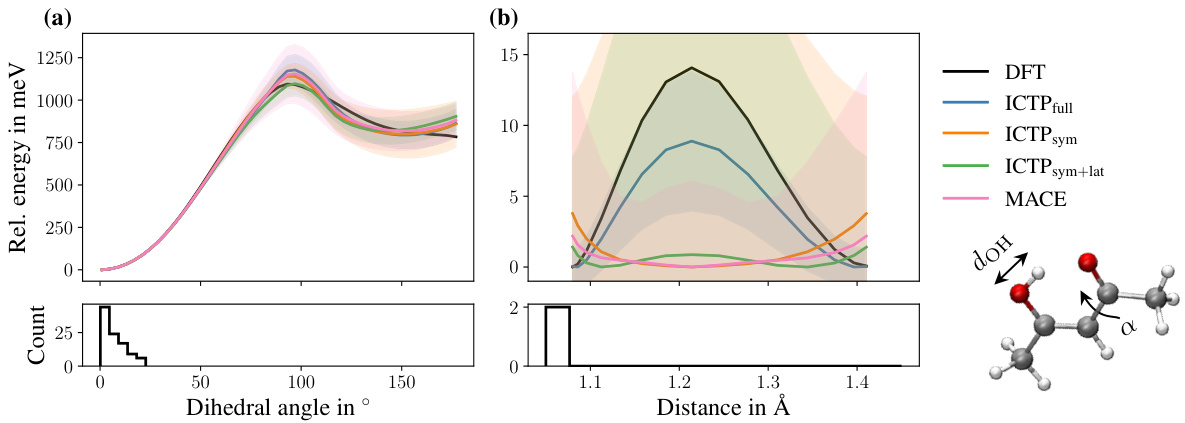
🔼 This figure compares the potential energy profiles of several MLIPs (including ICTP variants and MACE) against the reference DFT calculation for three different dihedral angles of the 3BPA molecule. Each plot shows the relative energy as a function of the dihedral angle or distance. The shaded region represents the standard deviation across five runs, demonstrating the models’ consistency. The inset shows the 3BPA molecule with its dihedral angles labeled.
read the caption
Figure 3: Potential energy profiles for three cuts through the 3BPA molecule's potential energy surface. All models are trained using 50 configurations, and additional 50 are used for early stopping. The 3BPA molecule, including the three dihedral angles (α, β, and γ), provided in degrees °, is shown as an inset. The color code of the inset molecule is C grey, O red, N blue, and H white. The reference potential energy profile (DFT) is shown in black. Each profile is shifted such that each model's lowest energy is zero. Shaded areas denote standard deviations across five independent runs.
More on tables

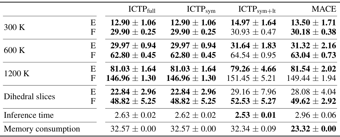
🔼 This table shows the RMSE of energy and force for different models trained on the 3BPA dataset. It compares the performance of ICTP (with various configurations) against MACE and NequIP, considering different temperatures and dihedral angles. Inference time and memory consumption are also reported, providing a holistic view of model efficiency.
read the caption
Table 2: Energy (E) and force (F) root-mean-square errors (RMSEs) for the 3BPA data set. E- and F-RMSE are given in meV and meV/Å, respectively. Results are shown for models trained using 450 configurations randomly drawn from the training data set collected at 300 K, with further 50 used for early stopping. All ICTP results are obtained by averaging over five independent runs. For MACE and NequIP, the results are reported for three runs. The standard deviation is provided if it is available. Best performances, considering the standard deviation, are highlighted in bold. Inference time and memory consumption are measured for a batch size of 100. Inference time is reported per structure in ms, while memory consumption is provided for the entire batch in GB.

🔼 This table shows the performance of different models on the 3BPA dataset. It presents the root-mean-square errors (RMSEs) for energy and force, calculated using different methods at three different temperatures (300 K, 600 K, and 1200 K) and along various dihedral angles. The table highlights the best performance achieved for each metric and condition and includes inference time and memory consumption.
read the caption
Table 2: Energy (E) and force (F) root-mean-square errors (RMSEs) for the 3BPA data set. E- and F-RMSE are given in meV and meV/Å, respectively. Results are shown for models trained using 450 configurations randomly drawn from the training data set collected at 300 K, with further 50 used for early stopping. All ICTP results are obtained by averaging over five independent runs. For MACE and NequIP, the results are reported for three runs. The standard deviation is provided if it is available. Best performances, considering the standard deviation, are highlighted in bold. Inference time and memory consumption are measured for a batch size of 100. Inference time is reported per structure in ms, while memory consumption is provided for the entire batch in GB.
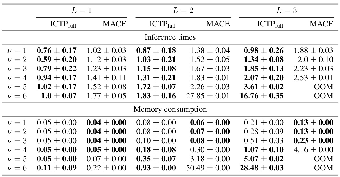
🔼 This table presents the inference times and memory consumption for ICTP and MACE models on the 3BPA dataset for different tensor ranks (L) and correlation orders (v). The results are averages over five independent runs, with standard deviations included where available. The table shows how the computational cost scales with increasing tensor rank and correlation order, highlighting the performance differences between the ICTP and MACE methods.
read the caption
Table A1: Inference times and memory consumption as a function of the tensor rank L and the correlation order v for the 3BPA data set. All values for ICTP and MACE models are obtained by averaging over five independent runs. The standard deviation is provided if it is available. Best performances are highlighted in bold. Inference time and memory consumption are measured for a batch size of 10. Inference time is reported per structure in ms; memory consumption is provided for the entire batch in GB.

🔼 This table presents the mean absolute errors (MAE) for energy (E) and force (F) in the MD22 dataset using various machine learning models, including the ICTP model proposed in this paper. The models were trained with the same dataset sizes as used in the original MD22 publication. The results highlight that the ICTP model performs on par with or better than other state-of-the-art models for this particular dataset.
read the caption
Table A2: Energy (E) and force (F) mean absolute errors (MAEs) for the MD22 data set.a E- and F-MAE are given in meV/atom and meV/Å, respectively. Results are shown for models trained using training set sizes defined in the original publication [48]. All values for ICTP models are obtained by averaging over three independent runs. We also use an additional subset of 500 configurations drawn randomly from the original data set for early stopping. The standard deviation is provided if available. Best performances, considering the standard deviation, are highlighted in bold.
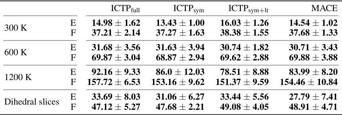
🔼 This table presents the RMSEs in total energies and atomic forces for the 3BPA dataset when training models with only 50 configurations. It compares the performance of ICTPfull, ICTPsym, ICTPsym+lt, and MACE models. The best performing model for each metric is highlighted.
read the caption
Table A3: Energy (E) and force (F) root-mean-square errors (RMSEs) for the 3BPA data set (results for Ntrain = 50). E- and F-RMSE are given in meV and meV/Å, respectively. Results are shown for models trained using 50 molecules randomly drawn from the training data set collected at 300 K, with further 50 used for early stopping. All ICTP and MACE results are obtained by averaging over five independent runs, with the standard deviation provided if available. Best performances, considering the standard deviation, are highlighted in bold.
🔼 This table presents the RMSEs in total energies and atomic forces for the 3BPA dataset when the models are trained with only 50 configurations. The table compares the performance of ICTP full, ICTP sym, ICTP sym+lt, and MACE models, showing the mean and standard deviation of the RMSEs for different temperatures and dihedral slices. It highlights the best performing models for each metric.
read the caption
Table A3: Energy (E) and force (F) root-mean-square errors (RMSEs) for the 3BPA data set (results for Ntrain = 50). E- and F-RMSE are given in meV and meV/Å, respectively. Results are shown for models trained using 50 molecules randomly drawn from the training data set collected at 300 K, with further 50 used for early stopping. All ICTP and MACE results are obtained by averaging over five independent runs, with the standard deviation provided if available. Best performances, considering the standard deviation, are highlighted in bold.

🔼 This table presents the RMSEs in total energies and atomic forces for the 3BPA dataset when models are trained with only 50 configurations. The results are compared for ICTP (with full, symmetric, and latent-space product basis) and MACE models at different temperatures (300 K, 600 K, 1200 K) and for dihedral angle slices. The best-performing model for each scenario is highlighted.
read the caption
Table A3: Energy (E) and force (F) root-mean-square errors (RMSEs) for the 3BPA data set (results for Ntrain = 50). E- and F-RMSE are given in meV and meV/Å, respectively. Results are shown for models trained using 50 molecules randomly drawn from the training data set collected at 300 K, with further 50 used for early stopping. All ICTP and MACE results are obtained by averaging over five independent runs, with the standard deviation provided if available. Best performances, considering the standard deviation, are highlighted in bold.

🔼 Table A6 presents the RMSEs in energy and force for the Ta-V-Cr-W dataset. It compares the performance of ICTP models with varying tensor ranks (L=0,1,2) against MACE models with the same tensor ranks, and also against MTP, GM-NN, and EAM. Results are shown separately for various subsystems (binary, ternary, quaternary alloys, and deformed structures) and overall. The table includes inference time and memory consumption per atom and per batch, respectively.
read the caption
Table A6: Energy (E) and force (F) root-mean-square errors (RMSEs) for the Ta-V-Cr-W data set. E- and F-RMSEs are given in meV/atom and eV/Å, respectively. Results are obtained by averaging over ten splits of the original data set, except for the deformed structures. For the latter, the results are obtained using the whole data set (training + test). For the ICTP, MACE, and GM-NN models, we randomly selected a validation data set of 500 structures from the corresponding training data sets. Best performances, considering the standard deviation, are highlighted in bold. Inference time and memory consumption are measured for a batch size of 50. Inference timea is reported per atom in µs; memory consumption is provided for the entire batch in GB.
Full paper#
