↗ OpenReview ↗ NeurIPS Homepage ↗ Chat
TL;DR#
Modern deep learning models frequently produce overconfident predictions, failing to accurately reflect uncertainty. This is particularly problematic in high-stakes applications where accurate uncertainty quantification is crucial. Existing calibration techniques often struggle to balance accuracy and calibration, leading to inconsistent optimization of these two objectives. The problem is further compounded by the variability in gradient magnitudes during training, potentially hindering the learning process.
This research introduces a novel approach that leverages a proportional-integral-derivative (PID) controller to dynamically adjust a probability-dependent gradient decay rate. The PID controller uses feedback from a relative calibration error metric to regulate the decay rate, maintaining a balance between accuracy and calibration. To address the issue of variable gradient magnitudes, an adaptive learning rate mechanism is implemented. Extensive experiments demonstrate the effectiveness of this method in consistently improving both accuracy and calibration, offering a significant advancement in model calibration techniques.
Key Takeaways#
Why does it matter?#
This paper is important because it addresses the critical issue of model miscalibration in deep learning, a problem that affects many applications. The proposed PID controller-based approach offers a novel solution to this problem, improving both model accuracy and calibration consistently. This work also opens up new avenues for research in adaptive optimization and uncertainty quantification in machine learning.
Visual Insights#

This figure shows curves illustrating how the gradient magnitude changes with increasing prediction probability (pc) for different values of the gradient decay hyperparameter (β). Each curve represents a different β value. The x-axis represents the prediction probability, and the y-axis represents the gradient magnitude. The figure demonstrates that as the prediction probability increases, the gradient magnitude decreases, and this decrease is more pronounced for larger values of β. This illustrates the effect of the probability-dependent gradient decay mechanism used in the proposed method, where the gradient is reduced more strongly for higher confidence predictions.
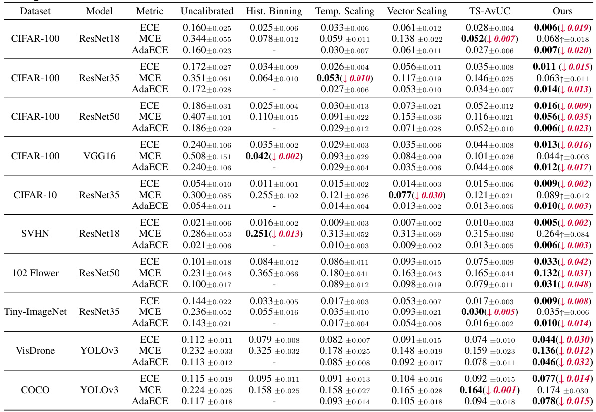
This table presents a comparison of the calibration performance of several post-hoc calibration methods against the proposed method. The metrics used are ECE, MCE, and AdaECE, calculated across different datasets and models. The best-performing method for each metric and dataset/model combination is highlighted in bold, with relative improvements over the second-best method shown in red. The results are averaged over five independent runs to ensure statistical robustness.
In-depth insights#
PID Calibration#
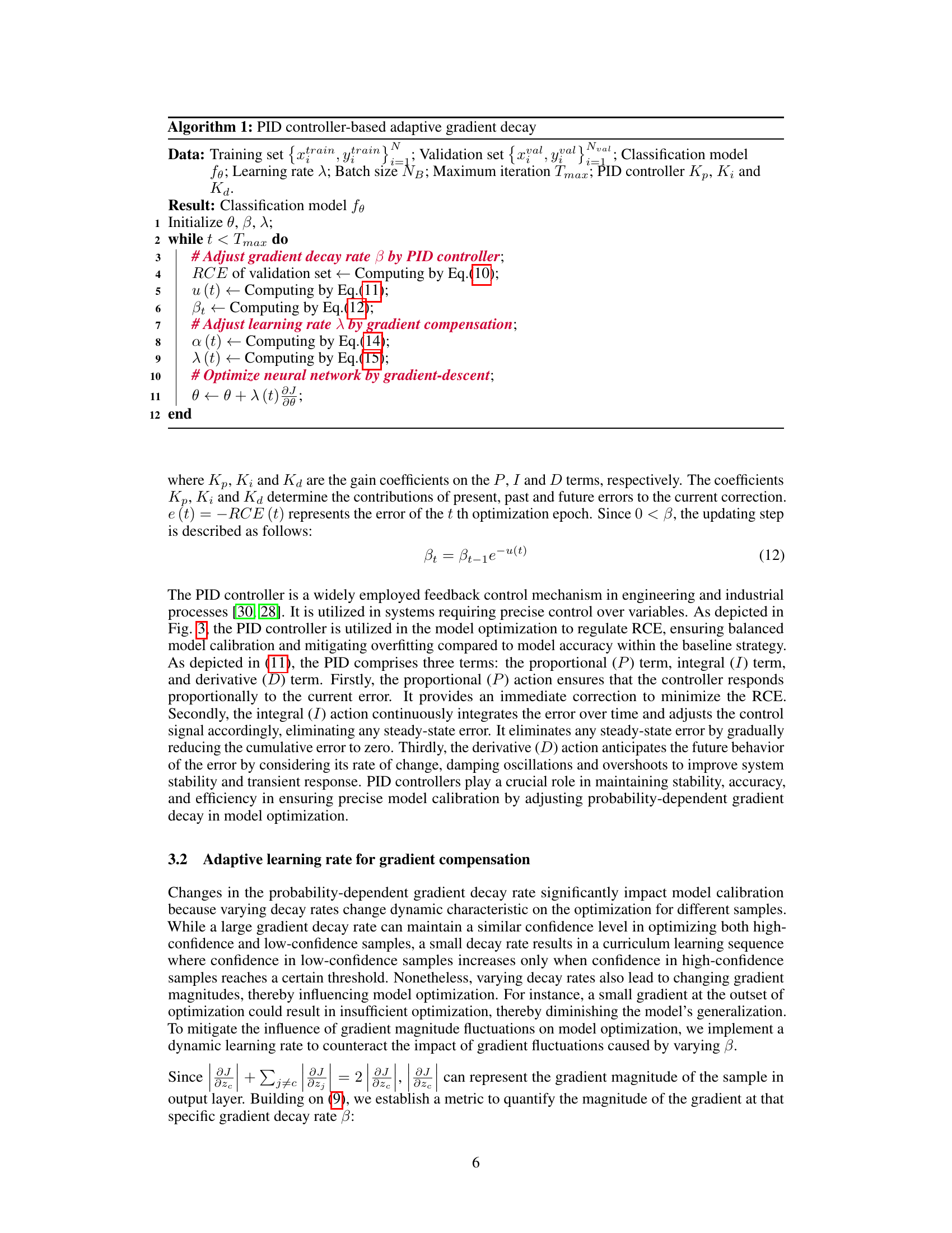
PID calibration, in the context of model calibration, presents a novel approach to adaptively manage gradient decay during model training. The core idea revolves around using a PID controller to dynamically adjust a probability-dependent gradient decay rate. This addresses the challenge of balancing model accuracy and calibration, as the calibration error often overfits sooner than classification accuracy. The PID controller receives feedback on the relative calibration error and adjusts the decay rate accordingly, mitigating issues of over-confidence or under-confidence. This adaptive mechanism ensures consistent optimization of both accuracy and calibration. The inclusion of an adaptive learning rate further compensates for fluctuations in gradient magnitude caused by the variable decay rate. Overall, this approach offers a robust and principled method for improving model calibration, leveraging the feedback control mechanisms of a PID controller to achieve effective uncertainty quantification.
Adaptive Gradient Decay#
Adaptive gradient decay methods dynamically adjust the learning rate during training, typically reducing it as the model converges. This addresses challenges posed by traditional methods with a fixed learning rate, which can lead to oscillations or slow convergence. Probability-dependent adaptive gradient decay is a sophisticated variant that ties the decay rate to the model’s confidence in its predictions. This approach is particularly useful in addressing overconfident predictions frequently observed in deep learning models, leading to improved calibration. A PID controller mechanism is one technique used to effectively manage the adaptive gradient decay rate, adjusting it based on real-time feedback on model calibration. Dynamic learning rate schedules complement the adaptive gradient decay approach to further refine the optimization process by counteracting fluctuations in gradient magnitude. While conceptually elegant, the effectiveness and optimal parameter selection of these techniques require careful empirical investigation, and theoretical underpinnings remain an area for further exploration.
Dynamic Learning Rate#
The concept of a dynamic learning rate in the context of model calibration is crucial. A fixed learning rate can hinder optimization, especially when dealing with probability-dependent gradient decay where gradient magnitudes fluctuate significantly throughout training. The paper highlights how a static rate might lead to inadequate learning due to over-small or over-large gradients during different phases of calibration. By implementing a dynamic learning rate, the model adapts to these changes, effectively counteracting fluctuations and ensuring consistent optimization. This dynamic adjustment helps to maintain a balance between model accuracy and calibration, preventing overconfidence or underconfidence in predictions. The adaptive learning rate mechanism, therefore, plays a pivotal role in enhancing the overall efficacy of the proposed PID-based adaptive gradient decay method for model calibration.
Model Calibration#
Model calibration, a crucial aspect in machine learning, focuses on aligning a model’s predicted probabilities with the true likelihood of events. Improper calibration leads to overconfident or underconfident predictions, hindering the model’s reliability, especially in high-stakes applications. Various techniques exist to address this, including post-hoc methods that adjust probabilities after model training and in-training methods that integrate calibration into the learning process. The choice of method depends on factors like model complexity, dataset characteristics, and the desired level of calibration accuracy. Bayesian approaches offer a principled way to model uncertainty, but can be computationally expensive. Ensemble methods can also improve calibration, but may increase computational cost. The effectiveness of a calibration method is typically evaluated using metrics like Expected Calibration Error (ECE), which quantifies the difference between predicted and actual probabilities across different confidence levels. Ultimately, successful model calibration is essential for deploying trustworthy and reliable models in real-world scenarios.
Future Research#
Future research directions stemming from this PID controller-based adaptive gradient decay method could explore several avenues. A more rigorous theoretical framework is needed to explain the relationship between gradient decay rate and confidence distribution, moving beyond empirical observations. Investigating the impact of different optimizers and their compatibility with the adaptive learning rate mechanism warrants further study. Expanding the application to various other model architectures and datasets, beyond those tested, would bolster the generalizability of the findings. A more sophisticated control system might also improve the dynamic calibration process, particularly for complex scenarios or imbalanced datasets. Finally, exploring alternative calibration metrics or incorporating uncertainty quantification techniques could enhance the overall performance and reliability of model calibration, offering potentially improved real-world applications.
More visual insights#
More on figures
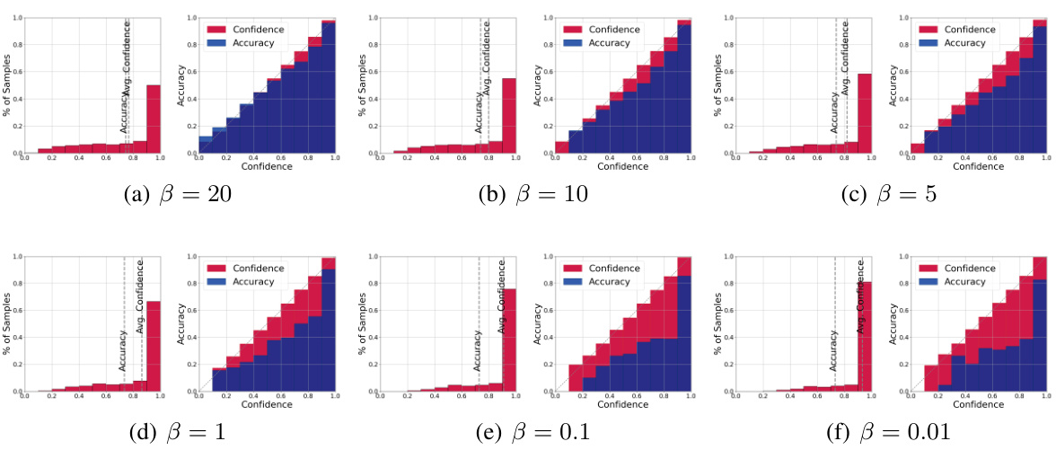
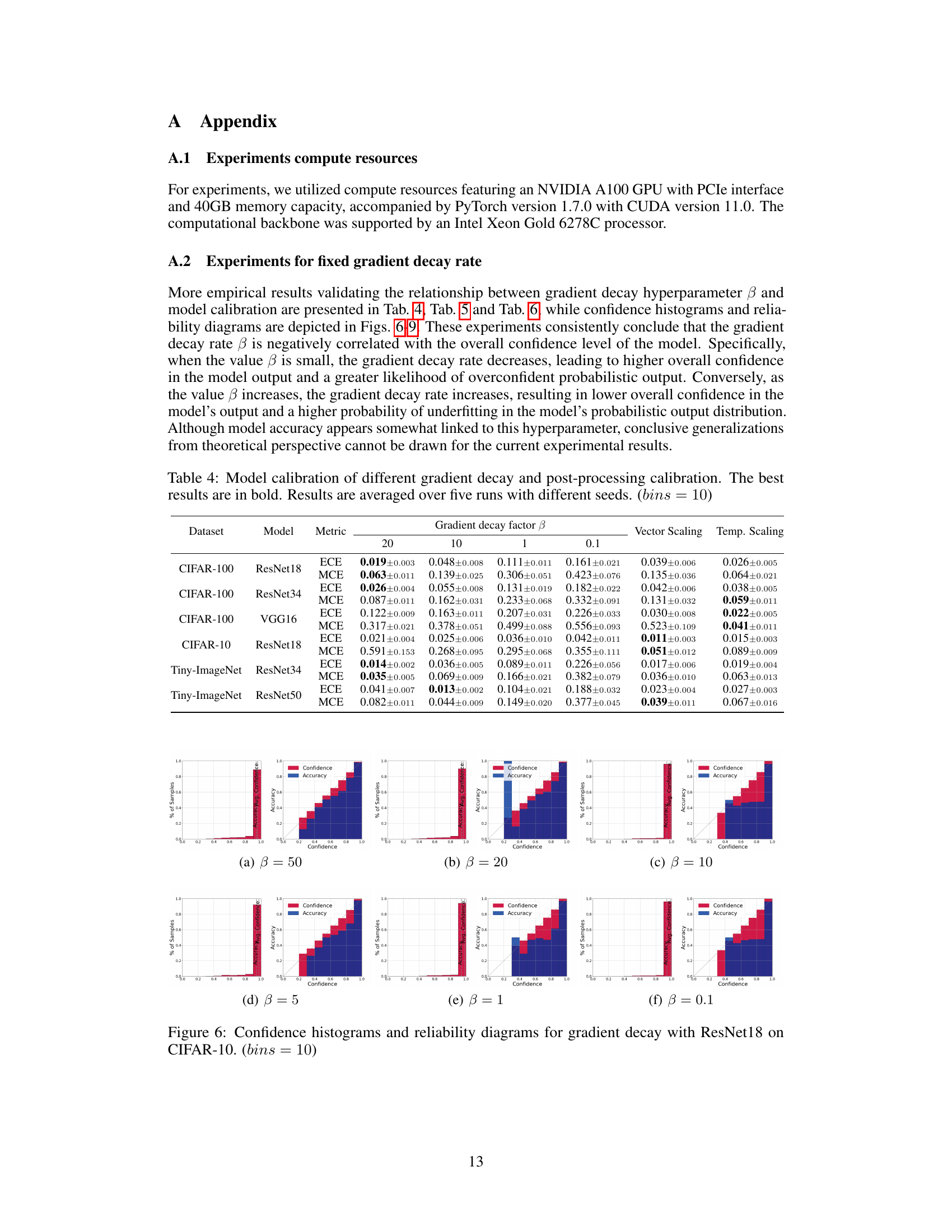
This figure visualizes the performance of ResNet18 on CIFAR-10 dataset under different gradient decay rates (β). Each subplot presents two plots: a confidence histogram showing the distribution of confidence scores and a reliability diagram illustrating the relationship between the average confidence and accuracy across different confidence intervals. The reliability diagram helps to assess the calibration of the model, while the confidence histogram shows the distribution of confidence levels. The figure demonstrates how varying the gradient decay rate impacts model calibration; the impact of the gradient decay rate on calibration is evident in the reliability diagrams.
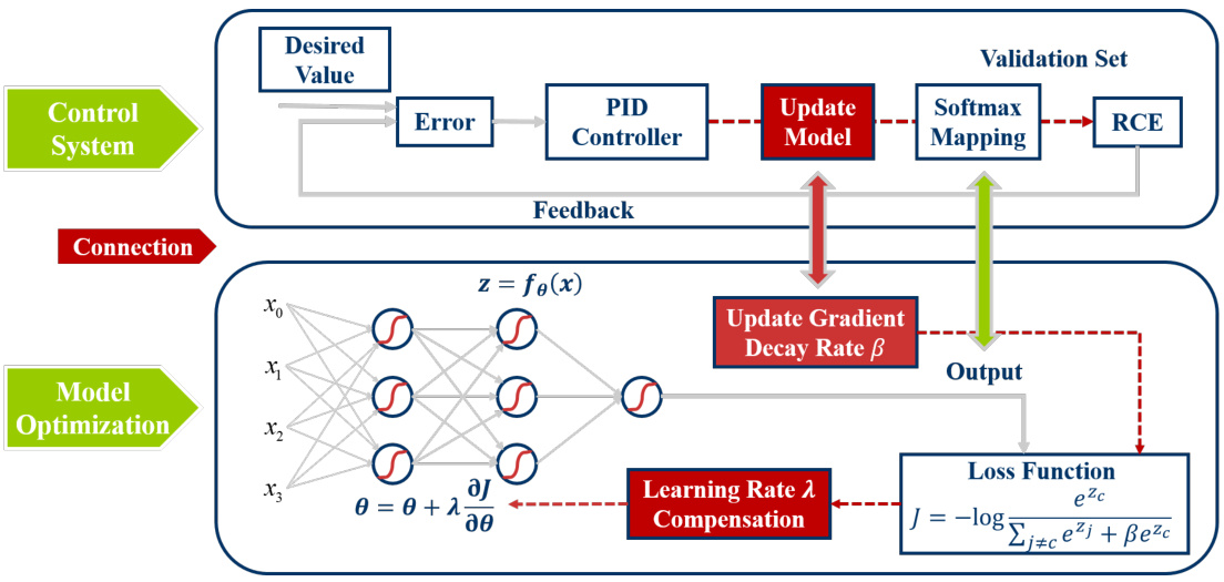
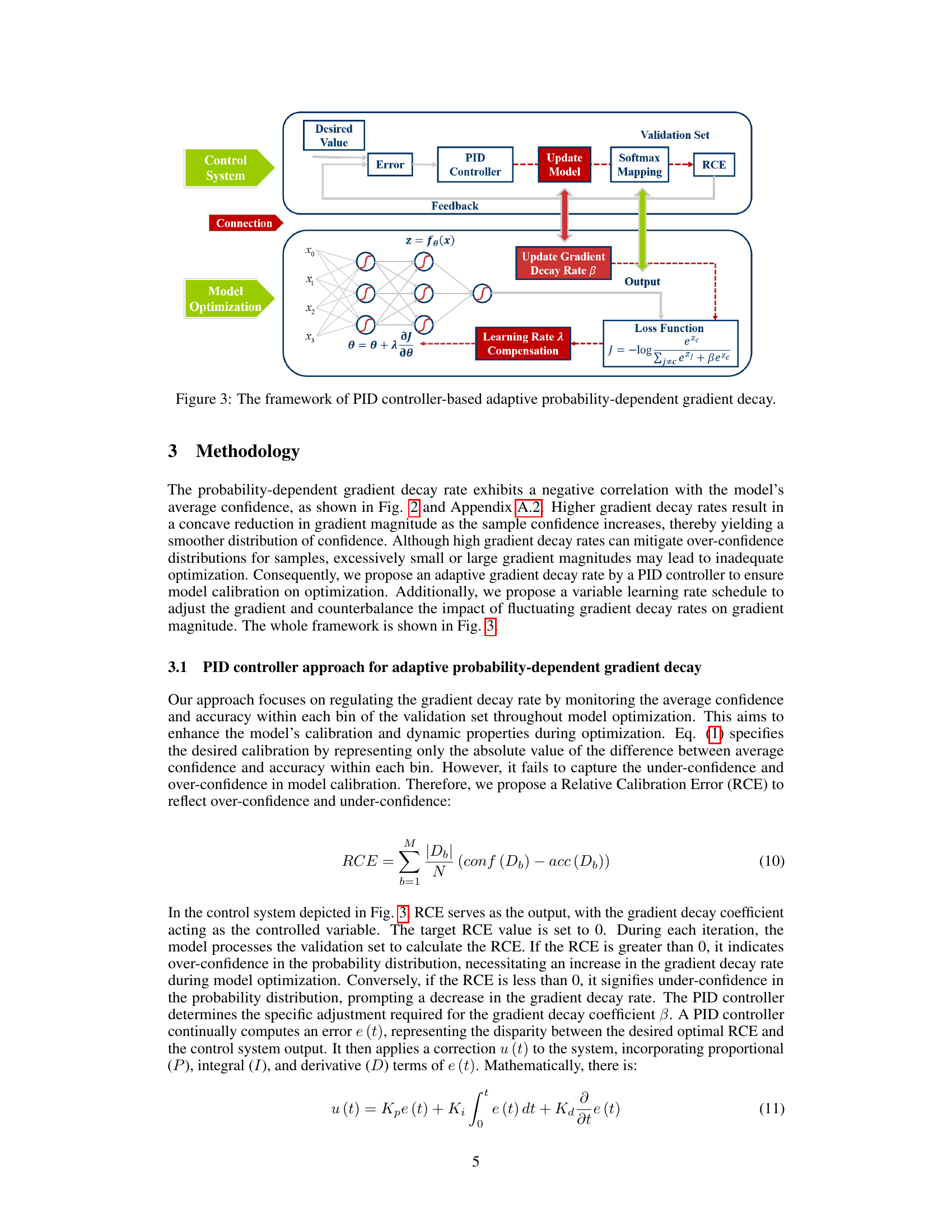
This figure illustrates the framework of the proposed PID controller-based adaptive probability-dependent gradient decay method. The control system uses the relative calibration error (RCE) calculated from a validation set as feedback. The RCE is compared to the desired value (0), and the difference (error) is used by a PID controller to adjust the gradient decay rate (β). This adjusted β is then used to update the model’s softmax mapping during the model optimization process. Simultaneously, a learning rate compensation mechanism is used to counterbalance the impact of fluctuating gradient decay rates on the gradient magnitude, ensuring stable and consistent model calibration and accuracy. The entire system aims to achieve a balance between optimizing model accuracy and its calibration.
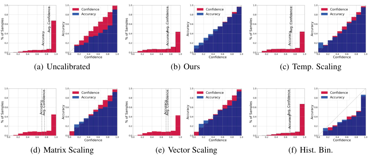
This figure compares the performance of different calibration methods (including the proposed PID controller approach) on the CIFAR-100 dataset using the ResNet35 model. Each subplot shows two plots: a histogram of the sample distribution across confidence bins and a reliability diagram showing the relationship between average confidence and accuracy within each bin. The ideal scenario is for the accuracy and confidence to match closely in each bin, indicating a well-calibrated model. The figure aims to visually demonstrate the effectiveness of the proposed method in improving model calibration, as indicated by better alignment between average confidence and accuracy compared to other methods.

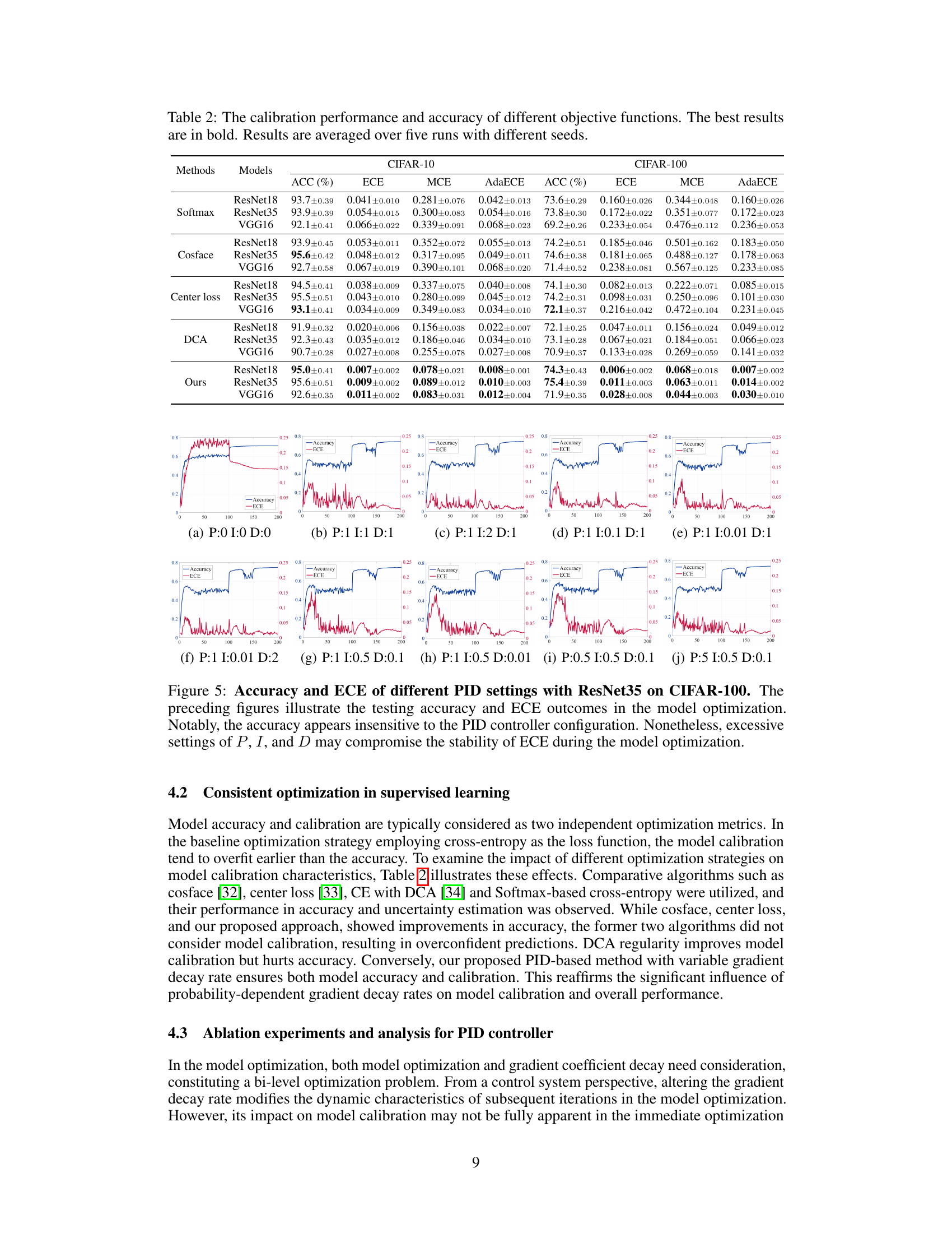
This figure shows the accuracy and expected calibration error (ECE) for different PID controller settings (proportional, integral, derivative gains) when training a ResNet35 model on the CIFAR-100 dataset. The results indicate that accuracy is relatively unaffected by the choice of PID settings, but that excessive settings can negatively impact the stability of the ECE. This highlights the importance of carefully tuning PID parameters to balance model accuracy and calibration.
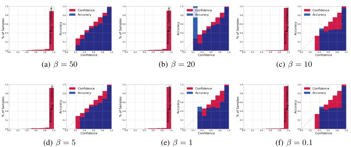
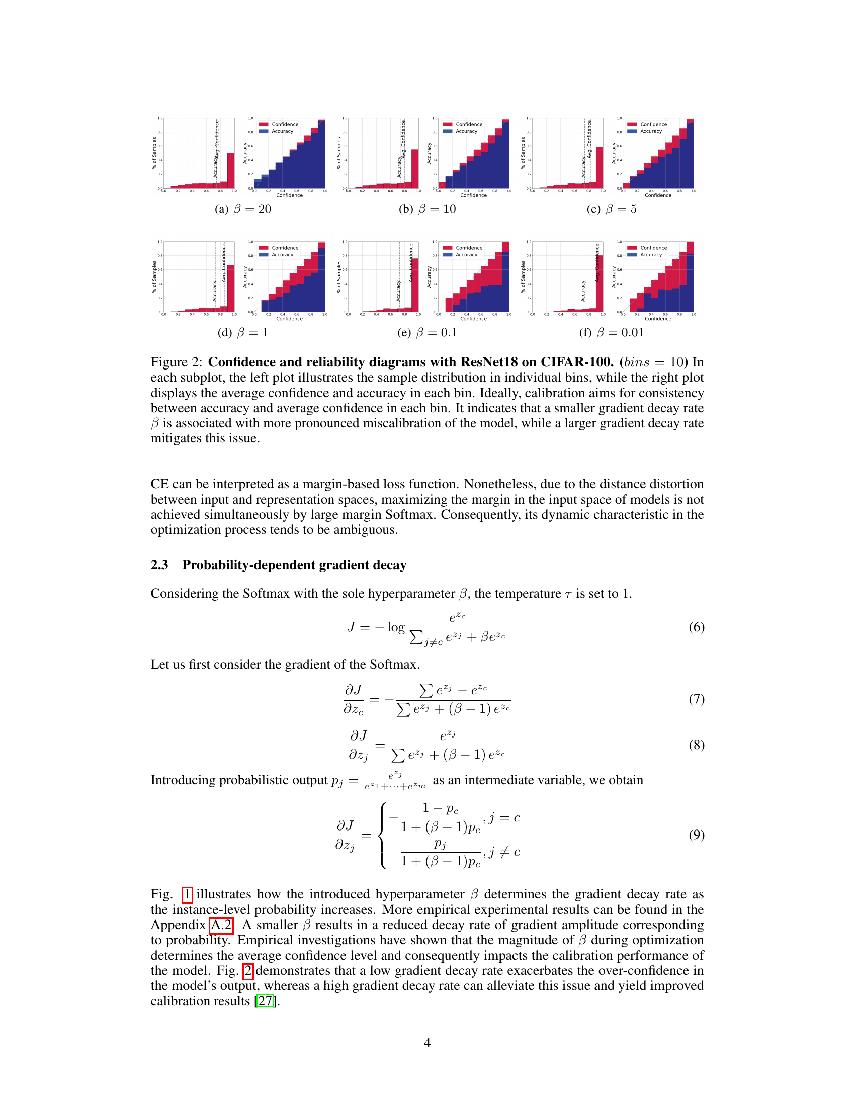
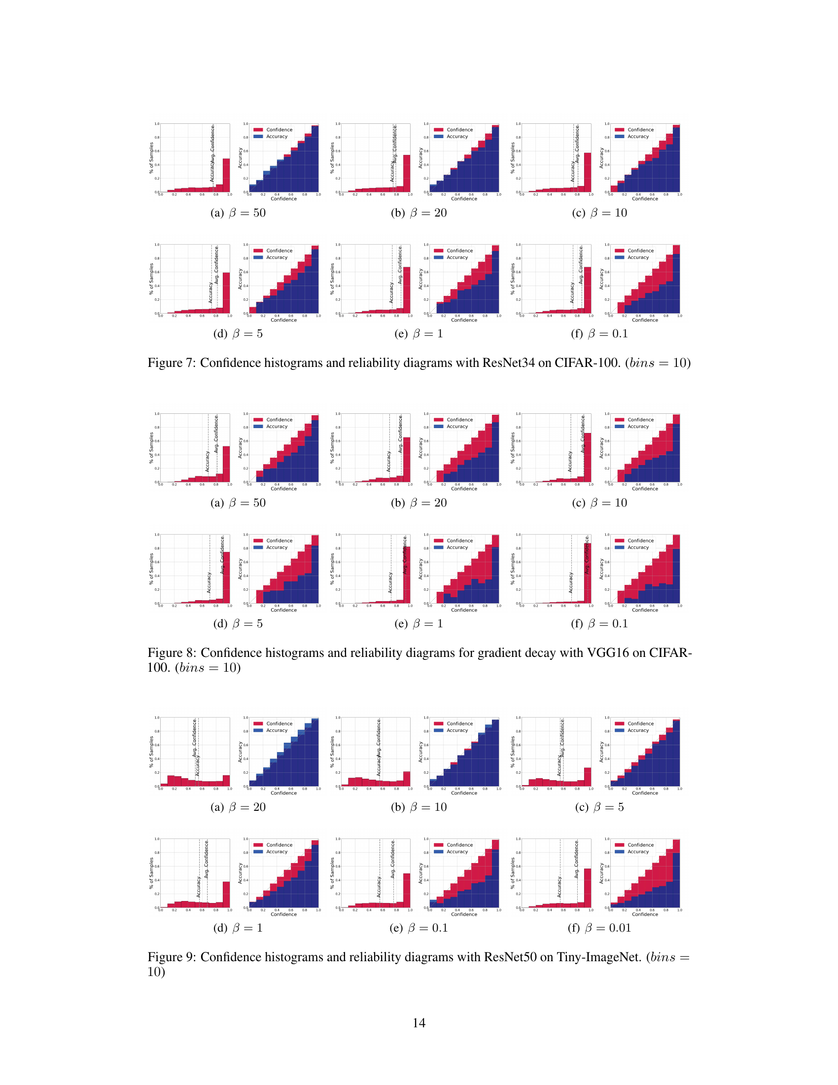
This figure shows the relationship between gradient decay rate (β) and model calibration performance using ResNet18 on the CIFAR-100 dataset. Each subplot displays both a histogram showing the distribution of samples across confidence bins and a reliability diagram comparing average confidence and accuracy within each bin. The results indicate that a smaller β leads to poorer calibration (overconfidence or underconfidence), while a larger β improves calibration.
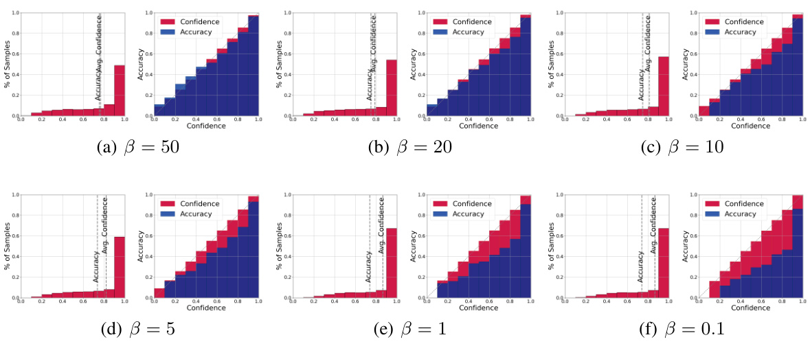
This figure shows the confidence and reliability diagrams for different gradient decay rates (β) using ResNet18 on the CIFAR-100 dataset. Each subplot contains two plots: a histogram showing the distribution of samples across confidence bins and a reliability diagram plotting the average confidence against the accuracy for each bin. The reliability diagrams illustrate the relationship between the model’s confidence and its actual accuracy. A perfectly calibrated model would show a diagonal line, indicating that the model’s confidence accurately reflects its predictive accuracy. Deviations from this diagonal line indicate miscalibration (overconfidence or underconfidence). The figure demonstrates that smaller values of β result in more miscalibration (larger deviation from the diagonal), while larger values lead to better calibration (closer to the diagonal).

This figure shows how the gradient magnitude changes with different gradient decay rates (β) as the probability (pc) increases. It illustrates the effect of the hyperparameter β on controlling the gradient decay rate within the Softmax function. A smaller β leads to a slower decay rate, while a larger β causes a faster decay, impacting the optimization process. The graph visually demonstrates the relationship between the hyperparameter, gradient magnitude, and the probability. This relationship is fundamental to the paper’s approach of adapting the gradient decay rate based on model confidence.

This figure shows the confidence and reliability diagrams for ResNet18 model trained on CIFAR-100 dataset. It visually represents the calibration performance of the model with different gradient decay rates (β). Each subplot presents a histogram showing the distribution of samples across confidence bins and a line plot illustrating average confidence versus accuracy for each bin. The ideal scenario shows perfect agreement between accuracy and average confidence, indicating perfect calibration. The figure demonstrates how smaller β values lead to worse miscalibration (larger discrepancy between accuracy and confidence), while larger values improve calibration.
More on tables

This table presents a comparison of different post-hoc calibration methods’ performance on various datasets and models. The metrics used for evaluation are ECE, MCE, and AdaECE. The best result for each metric and dataset/model combination is shown in bold, and the relative improvement compared to the second-best result is highlighted in red. The results are averaged over five independent runs, each using a different random seed, to ensure robustness and reliability.

This table compares the performance of different optimization algorithms (SGD and Adam) with and without the proposed PID controller approach and gradient compensation method. The results are evaluated on the ResNet35 model using the CIFAR-100 dataset. The metrics used for evaluation are accuracy, Expected Calibration Error (ECE), and Adaptive ECE (AdaECE).

This table presents the calibration performance results for different gradient decay factors (β) and post-processing calibration methods. The results are compared across various metrics (ECE, MCE) using different models (ResNet18, ResNet34, VGG16) and datasets (CIFAR-100, CIFAR-10, Tiny-ImageNet). The best performing method for each metric and dataset is highlighted in bold. The table illustrates how the choice of gradient decay factor impacts calibration performance and how it compares to established post-processing techniques.

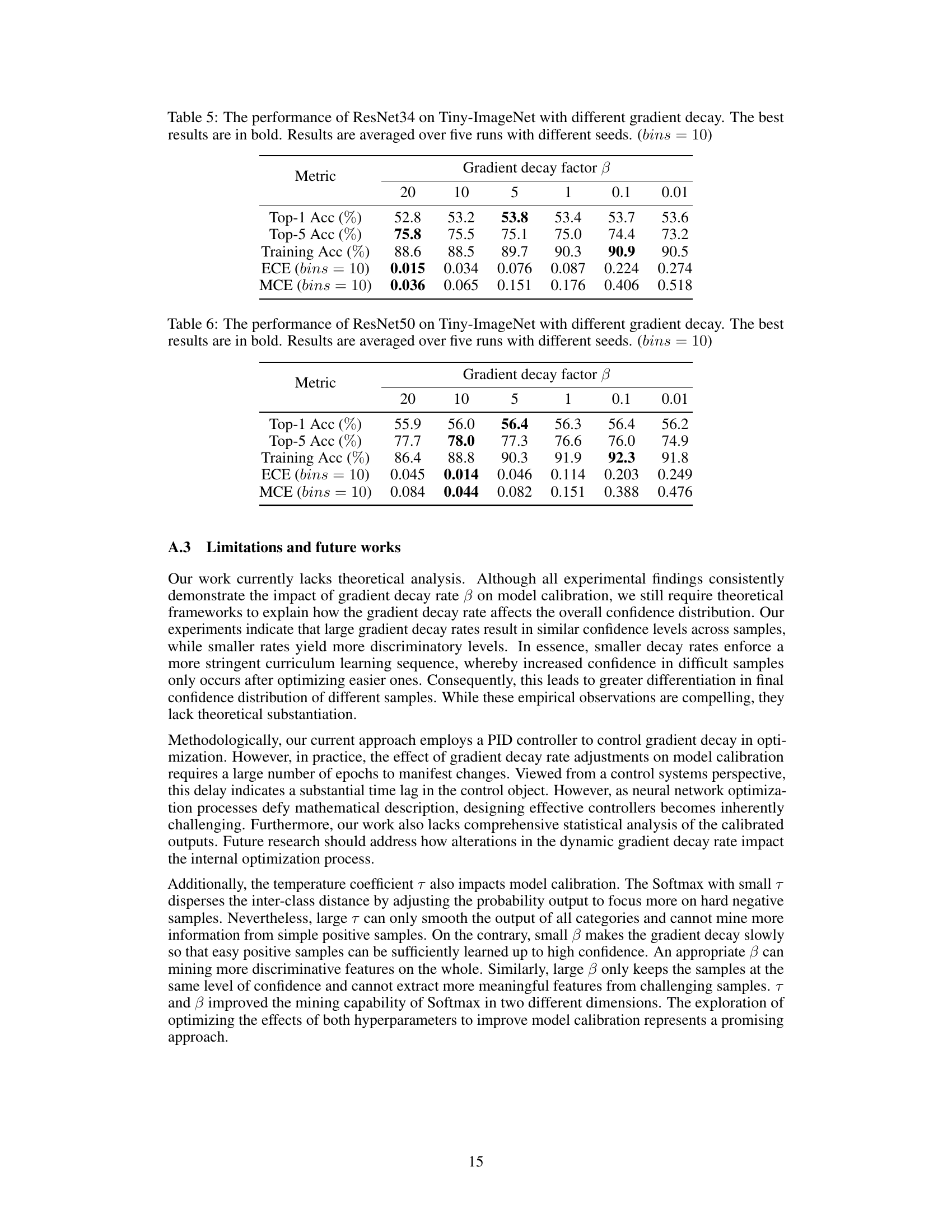
This table presents the performance of ResNet34 model on the Tiny-ImageNet dataset using different gradient decay factors (β). The metrics evaluated include Top-1 accuracy, Top-5 accuracy, training accuracy, Expected Calibration Error (ECE), and Maximum Calibration Error (MCE). The best results for each metric are highlighted in bold. The table shows how different gradient decay rates affect both the accuracy and calibration of the model, suggesting an optimal balance.
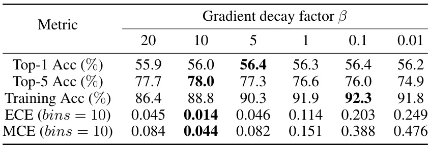
This table presents the performance of ResNet50 model on the Tiny-ImageNet dataset when using different gradient decay factors (β). It shows the impact of varying β on Top-1 accuracy, Top-5 accuracy, training accuracy, Expected Calibration Error (ECE), and Maximum Calibration Error (MCE). The best result for each metric is highlighted in bold. The experiment was repeated five times with different random seeds, and the average results are reported. The number of bins used in the ECE and MCE calculations is 10.
Full paper#
