TL;DR#
In-context learning, where LLMs solve tasks using only a few examples without explicit training, is a key paradigm. However, this paper reveals a significant limitation: LLMs often produce non-smooth and irregular decision boundaries, even on simple, linearly separable classification tasks. This means that small changes in input can lead to drastically different predictions, raising concerns about the reliability and generalizability of LLMs.
To address these issues, the researchers propose a new methodology: visualizing and analyzing decision boundaries. They investigate various factors influencing these boundaries, such as model size, prompt engineering, and fine-tuning techniques. Their experiments reveal that simply increasing the number of examples or model size doesn’t solve the problem. They explore methods such as training-free techniques, fine-tuning strategies, and active prompting methods, revealing that uncertainty-aware active learning can significantly improve decision boundary smoothness and overall performance.
Key Takeaways#
Why does it matter?#
This paper is crucial because it offers a novel way to understand in-context learning in LLMs, a very active area of research. By visualizing decision boundaries, it provides actionable insights into LLM behavior and suggests methods to improve model robustness and generalizability. This is important for advancing both theoretical and practical applications of LLMs.
Visual Insights#

🔼 This figure compares the decision boundaries produced by several large language models (LLMs) and traditional machine learning models on a simple, linearly separable binary classification task. The background color in each plot shows the model’s prediction for each region of the feature space, while the individual points represent the training or in-context examples provided to the model. The key observation is that the LLMs (LLama-3-8B and GPT-4) produce significantly less smooth, more irregular decision boundaries than the traditional models (Decision Tree, MLP, K-NN, SVM). This highlights a key difference in how LLMs and classical models approach the classification problem.
read the caption
Figure 1: Decision boundaries of LLMs and traditional machine learning models on a linearly separable binary classification task. The background colors represent the model's predictions, while the points represent the in-context or training examples. LLMs exhibit non-smooth decision boundaries compared to the classical models. See Appendix E for model hyperparameters.

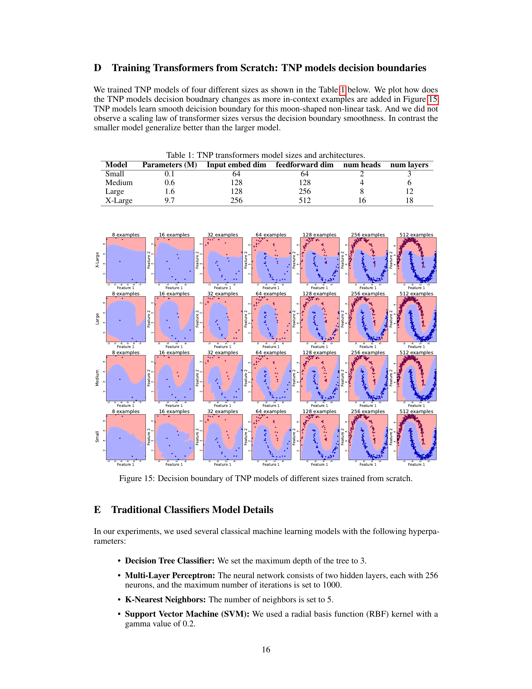
🔼 This table shows the different sizes of Transformer Neural Processes (TNP) models used in the experiments. Each model is defined by its number of parameters (in millions), input embedding dimension, feedforward dimension, number of heads, and number of layers. The models vary significantly in size and complexity, allowing for an analysis of how model scale affects the results.
read the caption
Table 1: TNP transformers model sizes and architectures.
In-depth insights#
LLM Decision Probes#
The heading ‘LLM Decision Probes’ suggests an investigation into the inner workings of large language models (LLMs). It likely involves probing the decision-making processes of LLMs, examining how they arrive at specific outputs given various inputs. This could entail analyzing the models’ responses to carefully designed prompts, or datasets, to understand their internal representations and reasoning mechanisms. The research likely aims to uncover biases, strengths, and weaknesses of LLMs by analyzing their decisions at a granular level. This may involve creating visualization techniques of the decision boundaries or employing methods from explainable AI (XAI) to interpret the reasoning path. Identifying patterns in the decision-making process could lead to insights regarding LLM behavior, prompting strategies, training methodologies, and even the inherent capabilities and limitations of this technology. Ultimately, this line of research is essential to enhance trust, reliability, and the responsible use of LLMs.
Boundary Irregularity#
The study reveals a significant and surprising finding regarding the decision boundaries produced by large language models (LLMs) in the context of classification tasks: irregularity and non-smoothness. This unexpected behavior challenges conventional understandings of LLM decision-making. Even in linearly separable tasks, where simpler models achieve smooth and predictable boundaries, LLMs struggle, revealing a complexity not anticipated. The research explores various factors, such as model size, dataset characteristics, and prompting techniques, and suggests that model size alone is insufficient to guarantee smooth boundaries. The investigation into decision boundary irregularity underscores the need for a deeper understanding of LLM inductive biases and how they impact generalization. It further highlights the potential implications of these findings for the reliability and robustness of LLM applications. The authors’ exploration of methods for improving boundary smoothness opens avenues for future research into improving LLM performance and understanding their emergent capabilities.
Impacting Factors#
Analyzing the paper’s findings on factors influencing in-context learning reveals several key insights. Model size, while intuitively expected to be a major factor, shows a complex relationship with performance. Larger models do not automatically translate to smoother decision boundaries, indicating that model architecture and training data also play crucial roles. The number of in-context examples significantly affects accuracy, but increasing their number does not guarantee smoother decision boundaries. The order of the in-context examples influences performance, highlighting the importance of careful prompt engineering. The level of quantization also impacts smoothness, suggesting that higher precision may be necessary for improved generalization. Finally, the prompt format and semantic characteristics of labels significantly affect the decision boundaries, demonstrating the complex interplay between linguistic factors and the underlying model behavior. Therefore, achieving robust and generalizable in-context learning requires a holistic approach considering the intricate interaction of these multiple factors.
Smoothing Methods#
The paper explores several techniques to enhance the smoothness of decision boundaries in large language models (LLMs). Fine-tuning emerges as a key method, with experiments evaluating the effects of fine-tuning different LLM layers (e.g., linear head, embedding layers, attention layers) and comparing fine-tuning on the in-context examples versus training on a broader dataset of classification tasks. The results highlight the importance of careful layer selection for fine-tuning to achieve smoother boundaries. Additionally, active learning strategies using uncertainty estimation are shown to improve sample efficiency and result in smoother boundaries. The comparison of active learning with random sampling showcases the benefits of the data-efficient and targeted approach. Quantization and prompt engineering (e.g., different label formats or example order) are also examined for their impact on boundary smoothness and model performance, revealing intricate relationships among these factors.
Future Directions#
Future research could explore scaling in-context learning to more complex tasks, moving beyond binary classification to encompass multi-class problems and real-world NLP applications. Investigating the impact of different prompt engineering techniques on decision boundary smoothness is crucial. Addressing the non-smoothness of decision boundaries observed in LLMs remains a key challenge and could involve novel architectural designs or training methods. A more thorough exploration of the relationship between model size, architecture, and decision boundary properties is warranted. It is vital to conduct a comprehensive analysis of how quantization and numerical precision influence the LLM’s decision-making process and its impact on generalization. Finally, developing more effective active learning strategies and exploring uncertainty-aware methods to guide data collection and improve sample efficiency are promising avenues for future research.
More visual insights#
More on figures

🔼 This figure compares the decision boundaries produced by six different LLMs (Sheared-Llama-1.3B, Llama-2-7B, Mistral-7B-v0.1, Llama-3-8B, GPT-3.5-turbo, and GPT-40) on a simple, linearly separable binary classification task. Each LLM was given 128 in-context examples. The background color represents the model’s prediction for each point in the feature space, while the scattered points represent the in-context examples themselves. The key observation is that all six LLMs produce irregular and non-smooth decision boundaries, in stark contrast to the smooth, well-defined boundaries expected from traditional machine learning models on this type of task. This illustrates a key finding of the paper: even state-of-the-art LLMs struggle to create smooth decision boundaries, regardless of model size.
read the caption
Figure 2: Visualizations of decision boundaries for various LLMs, ranging in size from 1.3B to 13B, on a linearly separable binary classification task. The in-context data points are shown as scatter points and the colors indicate the label determined by each model. These decision boundaries are obtained using 128 in-context examples. The visualization highlights that the decision boundaries of these language models are not smooth.

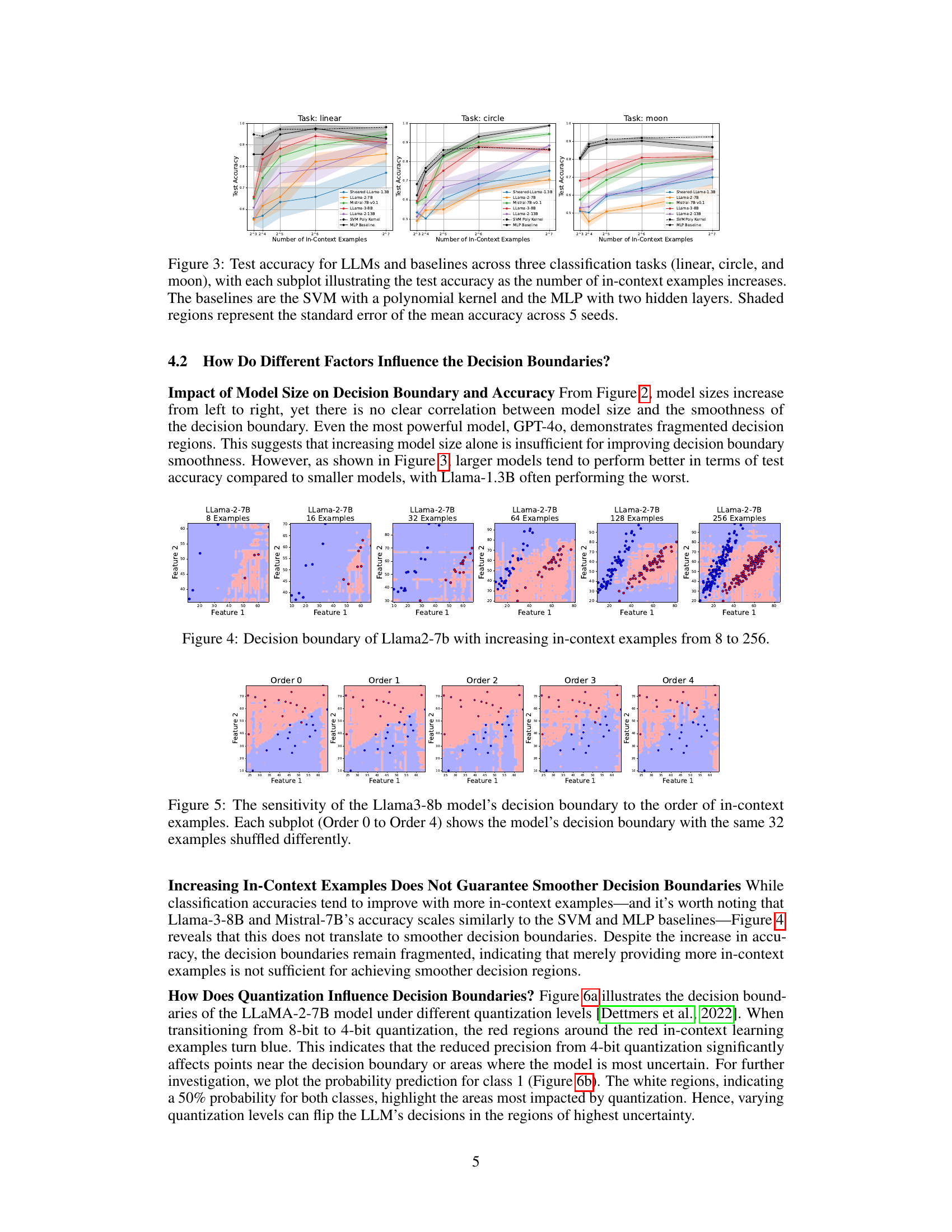
🔼 This figure displays the test accuracy of various LLMs and baseline models (SVM with polynomial kernel and MLP) across three different classification tasks (linear, circle, and moon) as the number of in-context examples increases. Each task represents a different level of complexity in terms of decision boundary shape. The shaded areas represent the standard error of the mean accuracy, providing a measure of the variability in the results. This allows for a comparison of how different models perform in terms of both accuracy and consistency as more examples are added. The x-axis represents the number of in-context examples (log scale), and the y-axis represents the test accuracy.
read the caption
Figure 3: Test accuracy for LLMs and baselines across three classification tasks (linear, circle, and moon), with each subplot illustrating the test accuracy as the number of in-context examples increases. The baselines are the SVM with a polynomial kernel and the MLP with two hidden layers. Shaded regions represent the standard error of the mean accuracy across 5 seeds.

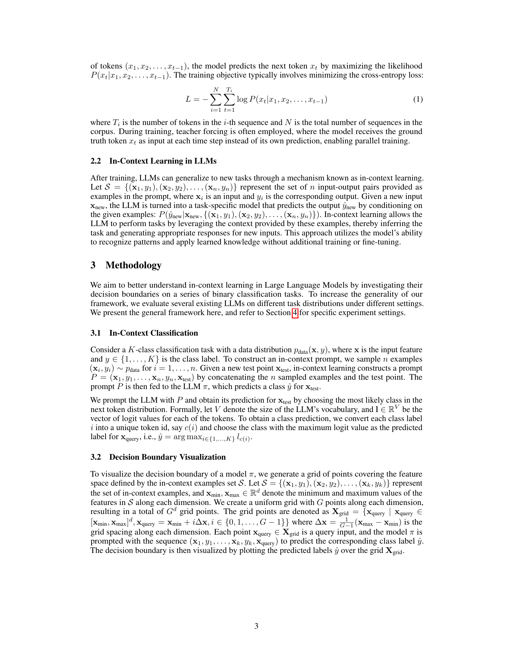
🔼 This figure visualizes the decision boundaries of the Llama2-7B language model on a binary classification task with varying numbers of in-context examples (8, 16, 32, 64, 128, and 256). Each subplot shows how the decision boundary changes as more examples are provided. The goal is to investigate whether increasing the number of examples leads to smoother and more generalized decision boundaries. The figure shows that even with a large number of examples, the decision boundaries remain irregular and non-smooth, indicating that simply increasing the number of in-context examples is not sufficient to improve the quality of the decision boundaries.
read the caption
Figure 4: Decision boundary of Llama2-7b with increasing in-context examples from 8 to 256.

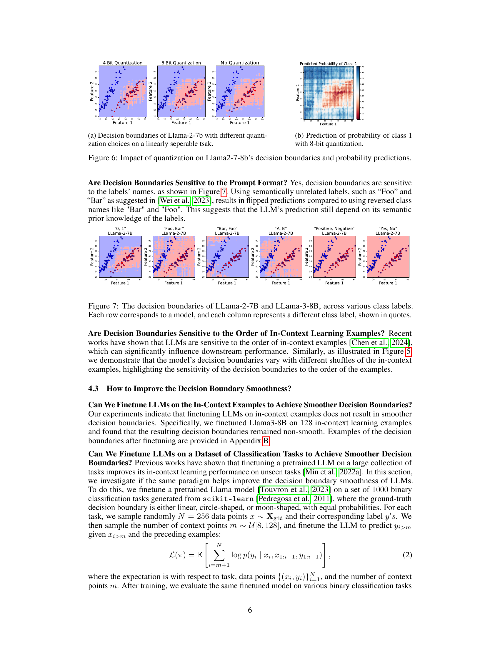
🔼 This figure visualizes how the order of in-context examples impacts the decision boundary generated by Llama-3-8b. Five subplots display the decision boundary for the same 32 examples but with different orderings (Order 0 through Order 4, presumably representing random shuffles). The variations in decision boundaries highlight the model’s sensitivity to the sequence of provided examples, suggesting that the order is a significant factor influencing in-context learning performance.
read the caption
Figure 5: The sensitivity of the Llama3-8b model's decision boundary to the order of in-context examples. Each subplot (Order 0 to Order 4) shows the model's decision boundary with the same 32 examples shuffled differently.

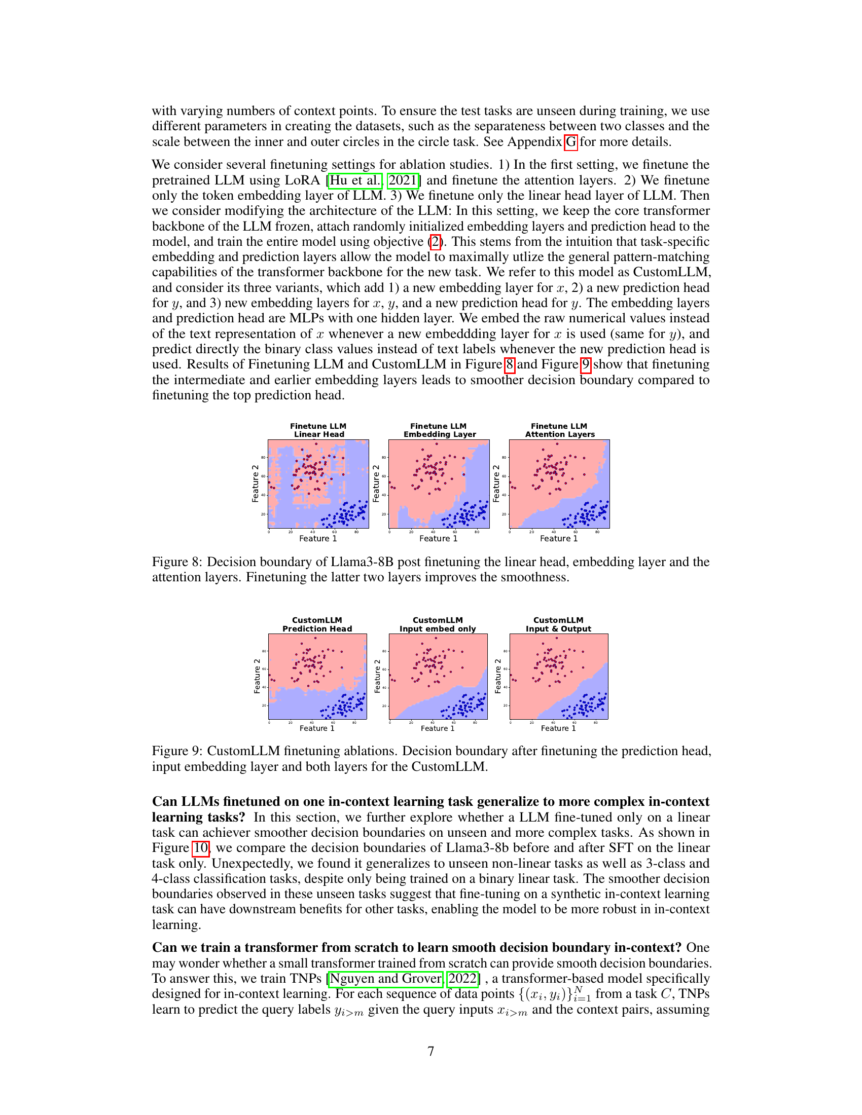
🔼 This figure shows the effect of different quantization levels (4-bit, 8-bit, and no quantization) on the decision boundaries and probability predictions of the Llama-2-7b language model. The left panels show the decision boundaries for a linearly separable task, illustrating how quantization affects the model’s ability to accurately classify data points, especially near the decision boundary. The right panel displays a heatmap visualizing the probability of class 1 under 8-bit quantization, highlighting regions of high uncertainty where quantization significantly impacts the model’s predictions.
read the caption
Figure 6: Impact of quantization on Llama2-7-8b's decision boundaries and probability predictions.

🔼 This figure visualizes the decision boundaries of two large language models (LLMs), Llama-2-7B and Llama-3-8B, on a binary classification task. The key point is how the decision boundaries change depending on the labels used in the prompt (e.g., ‘0, 1’, ‘Foo, Bar’, etc.). It demonstrates that the LLMs’ decision-making is not purely based on numerical values but also on the semantic understanding of the labels, showing a sensitivity to the choice of labels. The non-smooth, irregular boundaries are also noticeable.
read the caption
Figure 7: The decision boundaries of LLama-2-7B and LLama-3-8B, across various class labels. Each row corresponds to a model, and each column represents a different class label, shown in quotes.
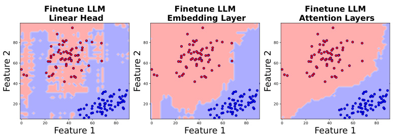
🔼 This figure compares the decision boundaries of Llama3-8B after fine-tuning different parts of the model (linear head, embedding layer, and attention layers) on a binary classification task. The goal was to see how fine-tuning these different components affects the smoothness of the decision boundary. The figure shows that fine-tuning the embedding layer and attention layers leads to a smoother decision boundary compared to fine-tuning only the linear head. This suggests that focusing on lower-level representations can be more effective in improving the generalization of in-context learning.
read the caption
Figure 8: Decision boundary of Llama3-8B post finetuning the linear head, embedding layer and the attention layers. Finetuning the latter two layers improves the smoothness.
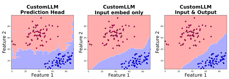
🔼 This figure shows the ablation study of the CustomLLM model’s performance in terms of the decision boundary smoothness. The model is fine-tuned on a binary classification task, and three different fine-tuning strategies are applied. The first one only finetunes the prediction head, the second one only finetunes the input embedding layer, and the third one finetunes both the prediction head and the input embedding layer. The resulting decision boundaries are visualized to compare the effectiveness of each fine-tuning strategy. The results indicate that finetuning both the prediction head and the input embedding layer yields the smoothest decision boundary, suggesting that both components play a crucial role in achieving good generalization performance.
read the caption
Figure 9: CustomLLM finetuning ablations. Decision boundary after finetuning the prediction head, input embedding layer and both layers for the CustomLLM.

🔼 This figure compares the decision boundaries produced by six different Large Language Models (LLMs) on a simple, linearly separable binary classification task. Each subfigure shows the decision boundary for a different LLM, ranging in size from 1.3B to 13B parameters. The background color represents the model’s prediction for each point in the feature space, while the scattered points represent the in-context examples used to guide the model’s learning. The key observation is that, despite the simplicity of the task and use of a substantial number of in-context examples, the decision boundaries are irregular and non-smooth, indicating limitations in the models’ ability to generalize.
read the caption
Figure 2: Visualizations of decision boundaries for various LLMs, ranging in size from 1.3B to 13B, on a linearly seperable binary classification task. The in-context data points are shown as scatter points and the colors indicate the label determined by each model. These decision boundaries are obtained using 128 in-context examples. The visualization highlights that the decision boundaries of these language models are not smooth.

🔼 This figure shows the decision boundaries produced by six different LLMs (Sheared-Llama-1.3B, Llama-2-7B, Mistral-7B-v0.1, Llama-3-8B, Llama-2-13B) on three types of binary classification tasks: circle, linear, and moon. Each model is given 128 in-context examples to learn from. The background color represents the model’s prediction for each point in the feature space, while the points themselves represent the in-context examples. The figure demonstrates that the decision boundaries of these LLMs are highly irregular and non-smooth, even on linearly separable tasks, unlike traditional machine learning models.
read the caption
Figure 12: Visualizations of decision boundaries for various LLMs, ranging in size from 1.3B to 13B, on three classification tasks. The tasks are, from top to bottom, circle, linear, and moon classifications. Note that the circle and moon tasks are not linearly separable. The in-context data points are shown as scatter points and the colors indicate the label determined by each model. These decision boundaries are obtained using 128 in-context examples. The visualization highlights that the decision boundaries of these language models are not smooth.
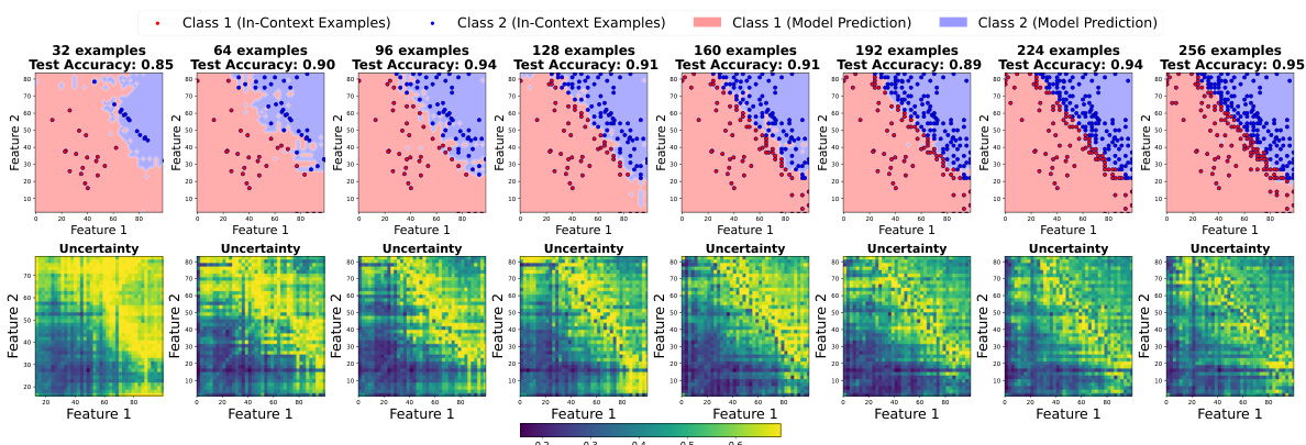
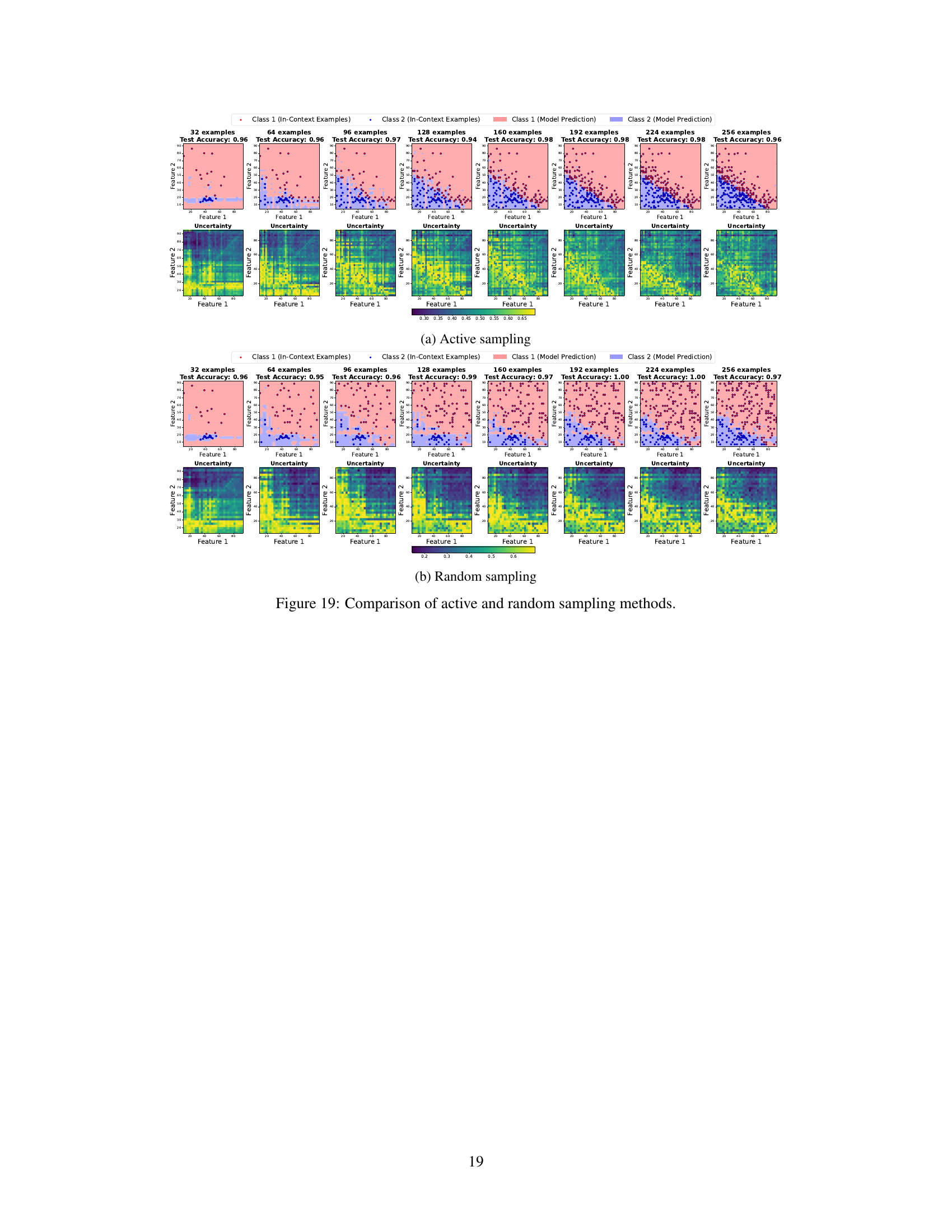
🔼 This figure compares the results of active and random sampling methods for improving the smoothness of decision boundaries in LLMs. It shows decision boundaries and uncertainty maps for a binary classification task. The left half displays the decision boundaries at different numbers of in-context examples (32-256) using active sampling, while the right half shows the same with random sampling. Active sampling focuses on selecting the most uncertain points to add as new examples, leading to progressively smoother and more accurate boundaries, as reflected by the higher test accuracies shown in the titles above each plot. The uncertainty maps show the regions where the model is most uncertain in its predictions, illustrating the effect of the sampling strategies.
read the caption
Figure 11: Comparison of active and random sampling methods. We plot the decision boundaries and uncertainty plot across different number of in-context examples from 32 to 256, where the in-context examples are gradually added to the prompt using active or random methods. Active sampling gives smoother decision boundary and the uncertain points lie on it. The test set accuracies is plotted in the titles.
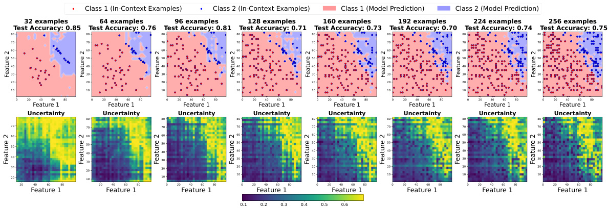
🔼 This figure compares active and random sampling methods for improving the smoothness of decision boundaries in LLMs. It shows how the decision boundary and uncertainty change as the number of in-context examples increases. Active sampling, which iteratively adds examples based on model uncertainty, leads to smoother boundaries and higher test accuracy compared to random sampling.
read the caption
Figure 11: Comparison of active and random sampling methods. We plot the decision boundaries and uncertainty plot across different number of in-context examples from 32 to 256, where the in-context examples are gradually added to the prompt using active or random methods. Active sampling gives smoother decision boundary and the uncertain points lie on it. The test set accuracies is plotted in the titles.

🔼 This figure displays the decision boundaries of six different LLMs on three different classification tasks: circle, linear, and moon. The background color represents the model’s prediction for each point, and the individual points represent the in-context examples used. The figure demonstrates that even on simple, linearly separable tasks (linear), the decision boundaries produced by the LLMs are irregular and non-smooth, unlike the smooth boundaries produced by traditional machine learning models. This irregular behavior highlights a key limitation of current LLMs’ in-context learning capabilities.
read the caption
Figure 12: Visualizations of decision boundaries for various LLMs, ranging in size from 1.3B to 13B, on three classification tasks. The tasks are, from top to bottom, circle, linear, and moon classifications. Note that the circle and moon tasks are not linearly separable. The in-context data points are shown as scatter points and the colors indicate the label determined by each model. These decision boundaries are obtained using 128 in-context examples. The visualization highlights that the decision boundaries of these language models are not smooth.
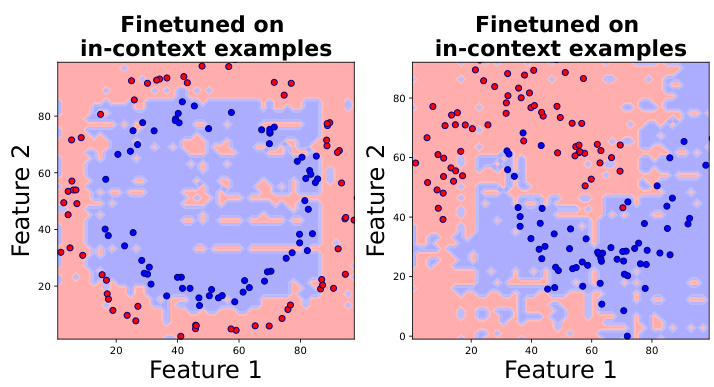
🔼 This figure shows the decision boundaries of Llama2-7B after finetuning on in-context examples. The background colors represent the model’s predictions, and the points represent the in-context examples used for finetuning. The decision boundaries are irregular, fragmented, and do not show a smooth separation between the two classes, even after finetuning. This illustrates that finetuning solely on in-context examples does not guarantee smoother or more generalizable decision boundaries.
read the caption
Figure 13: Two examples of Llama2-7B finetuned on the in-context examples points, which are scattered points in the plot.
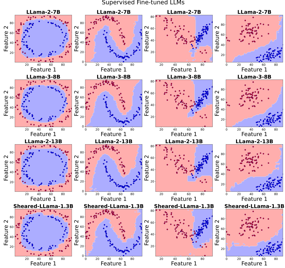
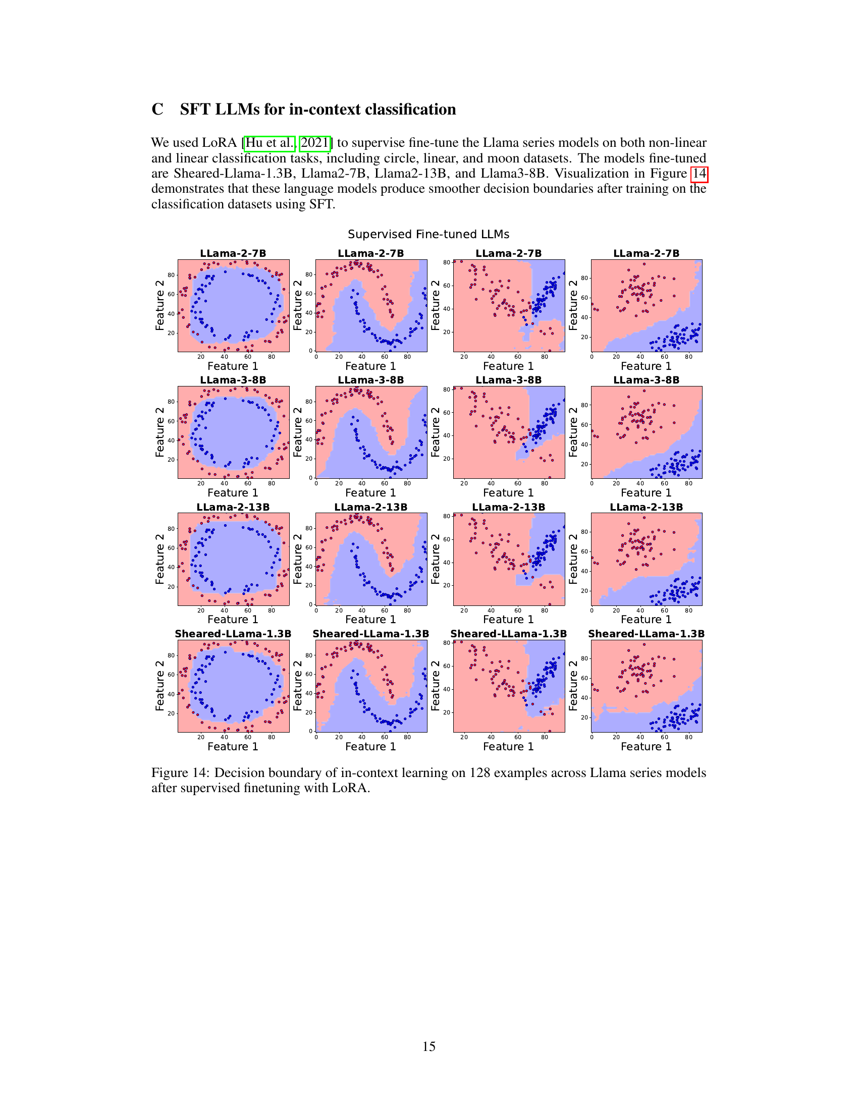
🔼 This figure displays the decision boundaries of several Llama language models after fine-tuning with LoRA on a task involving 128 in-context examples. Each row represents a different Llama model (Llama-2-7B, Llama-3-8B, Llama-2-13B, Sheared-Llama-1.3B), and each column shows the decision boundary visualization from a different angle/perspective. The images aim to demonstrate the impact of supervised fine-tuning with LoRA on the smoothness and regularity of the decision boundaries in the models, in comparison to the models’ performance before fine-tuning.
read the caption
Figure 14: Decision boundary of in-context learning on 128 examples across Llama series models after supervised finetuning with LoRA.
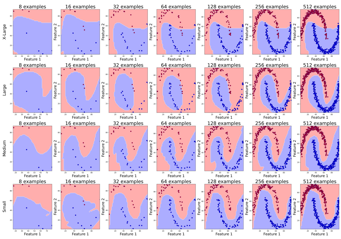
🔼 This figure visualizes the decision boundaries of Transformer Neural Process (TNP) models with varying sizes (small, medium, large, X-large) on a moon-shaped non-linear binary classification task. Each row represents a model size, and each column shows the decision boundary with an increasing number of in-context examples (8, 16, 32, 64, 128, 256, 512). The background color represents the model’s prediction, while the points represent the in-context examples. The visualization aims to illustrate how the decision boundary changes with the number of in-context examples and the effect of model size on boundary smoothness and generalization. Notably, the smaller model demonstrates better generalization than larger models in this specific scenario.
read the caption
Figure 15: Decision boundary of TNP models of different sizes trained from scratch.
🔼 This figure compares the decision boundaries produced by several large language models (LLMs) and traditional machine learning models on a simple, linearly separable binary classification task. The background color shows the model’s prediction for each point in the feature space. The individual points represent the in-context examples used to prompt the model. The key observation is that the LLMs produce irregular, non-smooth decision boundaries, in contrast to the smooth boundaries generated by the traditional classifiers. This illustrates a key finding of the paper: LLMs struggle with producing smooth and generalizable decision boundaries, even on simple tasks.
read the caption
Figure 1: Decision boundaries of LLMs and traditional machine learning models on a linearly separable binary classification task. The background colors represent the model's predictions, while the points represent the in-context or training examples. LLMs exhibit non-smooth decision boundaries compared to the classical models. See Appendix E for model hyperparameters.

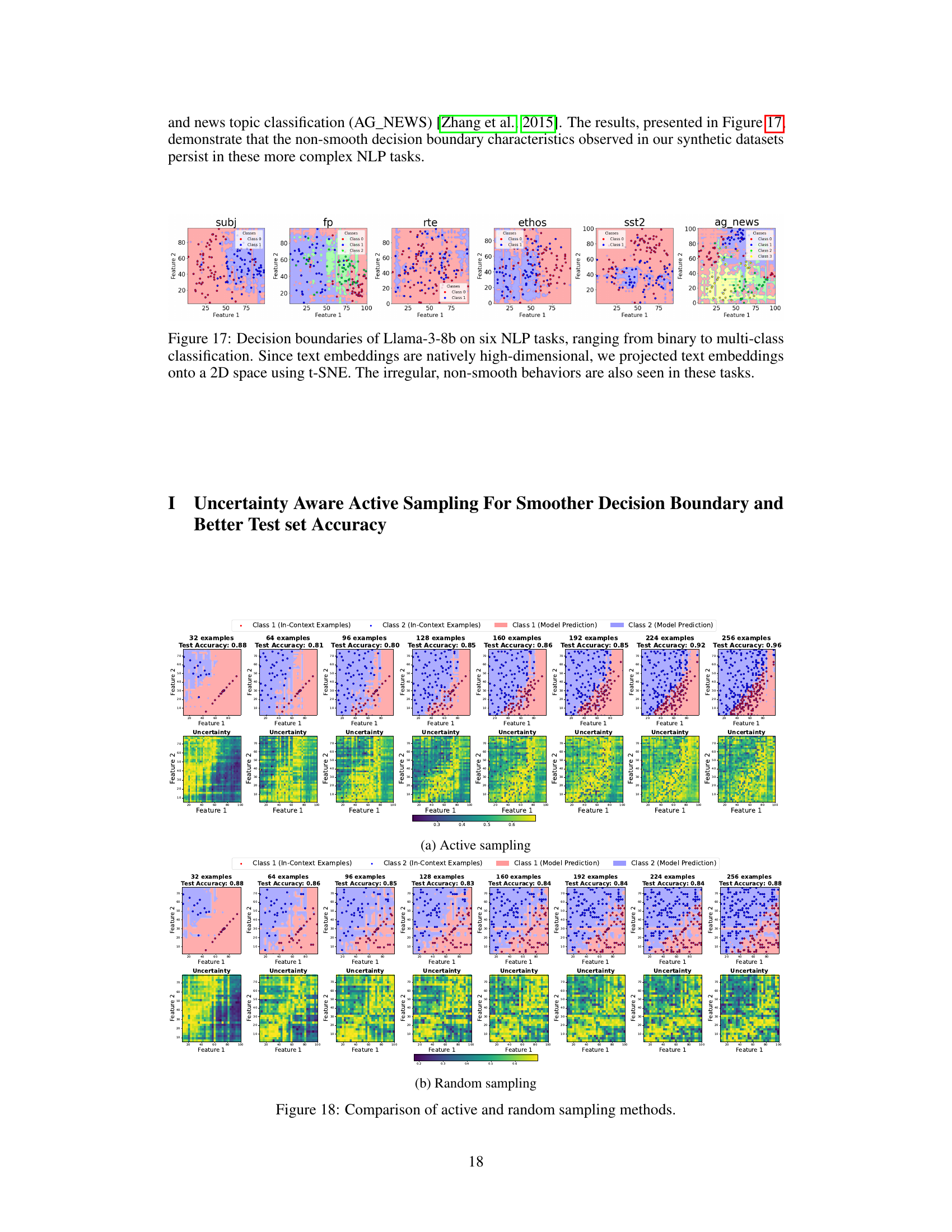
🔼 This figure visualizes the decision boundaries of the Llama-3-8B model on six different NLP tasks, ranging in complexity from binary to multi-class classification. Because text embeddings are high-dimensional, t-SNE dimensionality reduction was used to project them into 2D space for visualization. The visualization reveals that even on these real-world NLP tasks, the decision boundaries remain irregular and non-smooth, consistent with the observations made on simpler, synthetic tasks.
read the caption
Figure 17: Decision boundaries of Llama-3-8b on six NLP tasks, ranging from binary to multi-class classification. Since text embeddings are natively high-dimensional, we projected text embeddings onto a 2D space using t-SNE. The irregular, non-smooth behaviors are also seen in these tasks.

🔼 This figure compares the effectiveness of active and random sampling methods in improving the smoothness of decision boundaries and test set accuracy for Llama-3-8B. The top row shows the decision boundaries obtained using active sampling, where the model is queried on the most uncertain points to iteratively refine the boundary. The bottom row shows the results using random sampling. Each column represents a different number of in-context examples (32 to 256). The heatmaps in the bottom row show the uncertainty for each point (higher values indicate higher uncertainty). The plots demonstrate that active sampling consistently results in smoother boundaries and higher test accuracy than random sampling.
read the caption
Figure 11: Comparison of active and random sampling methods. We plot the decision boundaries and uncertainty plot across different number of in-context examples from 32 to 256, where the in-context examples are gradually added to the prompt using active or random methods. Active sampling gives smoother decision boundary and the uncertain points lie on it. The test set accuracies is plotted in the titles.
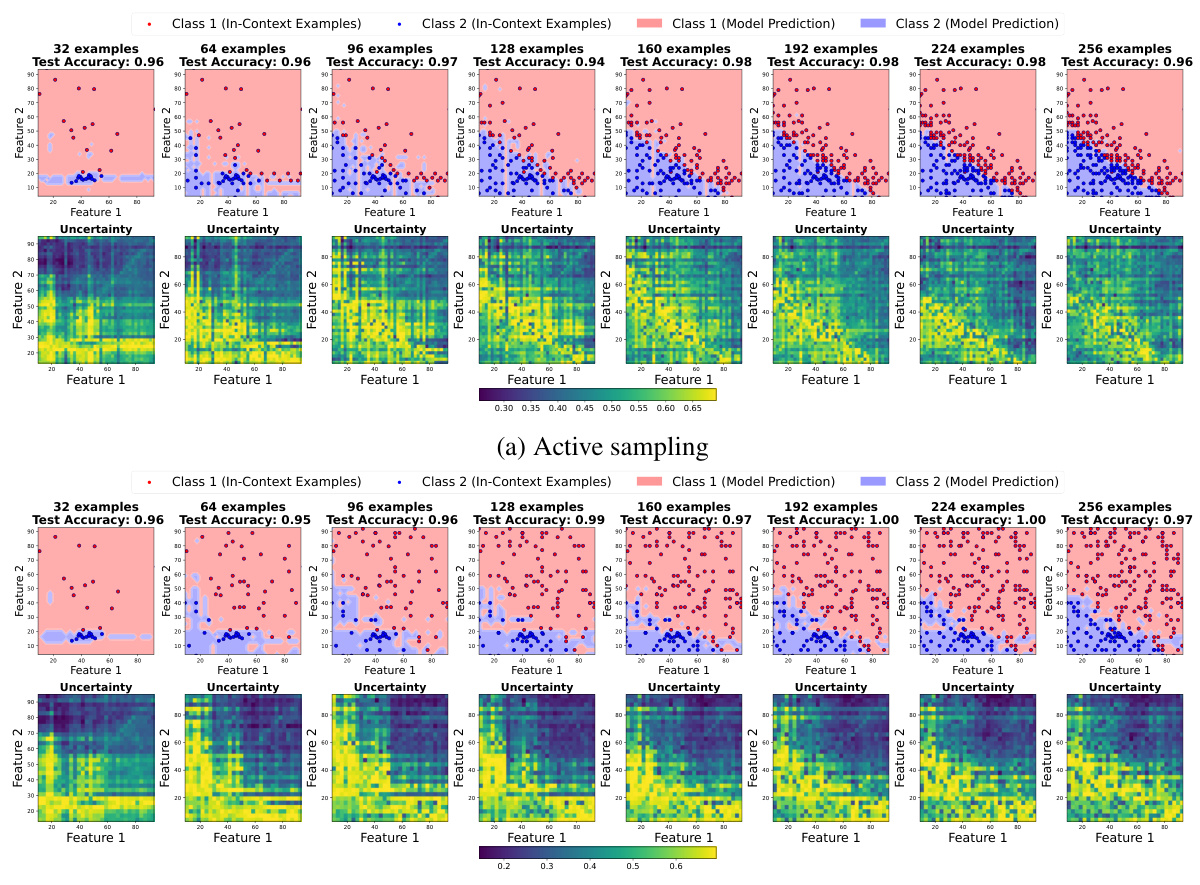
🔼 This figure compares the results of active and random sampling methods for improving the smoothness of decision boundaries in LLMs. It shows how the decision boundary changes as more in-context examples are added using both active (top) and random (bottom) sampling techniques. Each subplot displays the decision boundary and uncertainty heatmap for a specific number of in-context examples, ranging from 32 to 256. The active sampling method, which selectively adds the most uncertain points to the prompt, consistently generates smoother boundaries compared to random sampling. Test accuracies are reported for each subplot to illustrate the overall performance improvement gained through active learning.
read the caption
Figure 11: Comparison of active and random sampling methods. We plot the decision boundaries and uncertainty plot across different number of in-context examples from 32 to 256, where the in-context examples are gradually added to the prompt using active or random methods. Active sampling gives smoother decision boundary and the uncertain points lie on it. The test set accuracies is plotted in the titles.
Full paper#


