TL;DR#
Traditional neural network training assumes stationary data, but many real-world scenarios involve non-stationary data distributions (e.g., continual learning, reinforcement learning). This often leads to “plasticity loss,” where the model struggles to adapt to new data, hindering performance. Existing methods, such as hard resets, can be inefficient as they discard useful information.
This paper introduces Soft Resets, a novel learning method that addresses plasticity loss by modeling non-stationarity using an Ornstein-Uhlenbeck process with an adaptive drift. This drift mechanism gently nudges the model’s parameters toward their initial state, acting as a soft reset. Experiments demonstrate that Soft Resets significantly improves performance in non-stationary settings, outperforming baselines across various tasks including continual learning and reinforcement learning benchmarks.
Key Takeaways#
Why does it matter?#
This paper is crucial for researchers in machine learning, especially those working with non-stationary data. It introduces a novel approach to address plasticity loss, a significant challenge in continual learning and reinforcement learning, paving the way for more robust and adaptive AI systems. The method’s effectiveness across various tasks and its clear explanation make it valuable for both theoretical and practical advancements.
Visual Insights#

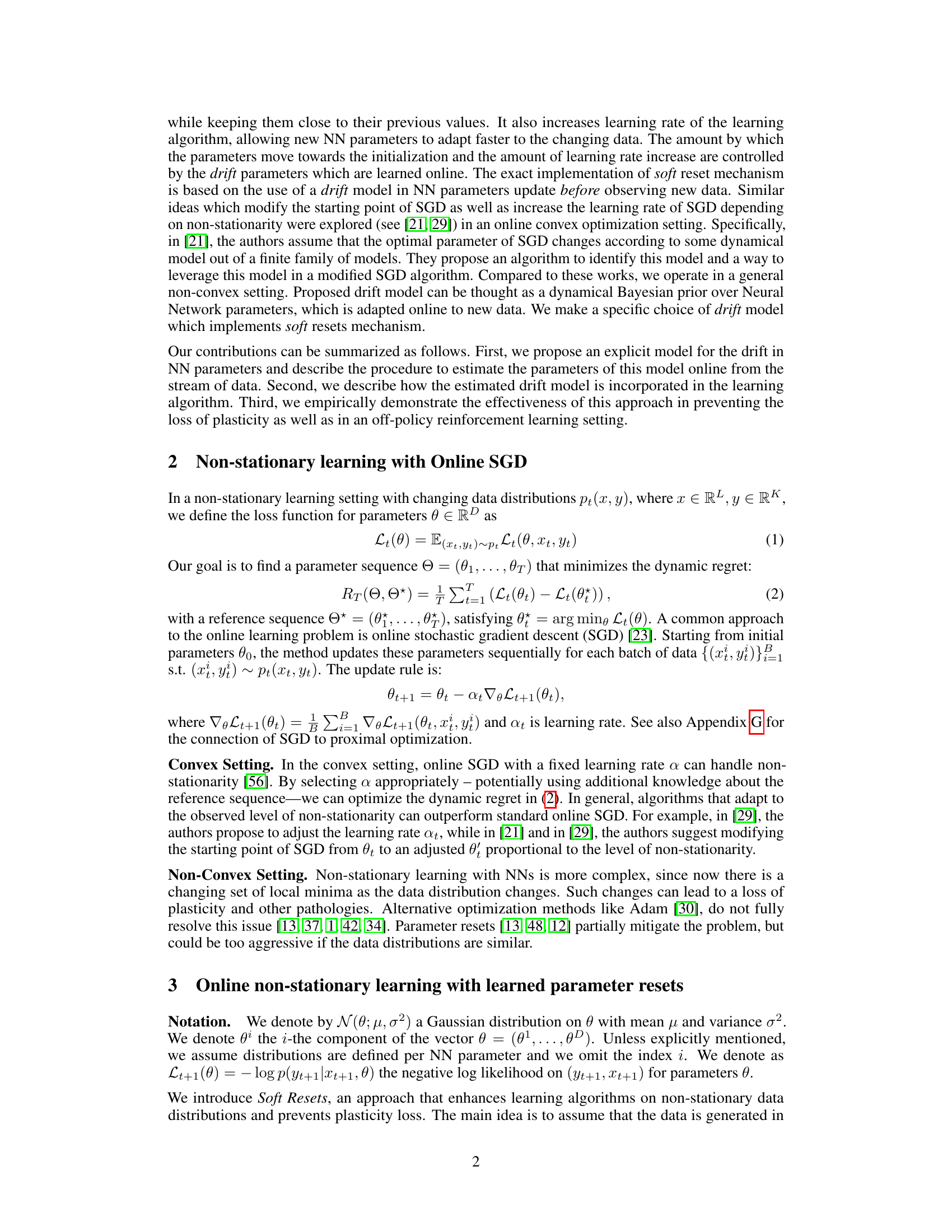
🔼 This figure visually explains the concept of soft parameter reset using a Bayesian inference example. The left side shows the graphical models for the data generating process under stationary (a) and non-stationary (b) assumptions. The right side illustrates how the Bayesian posterior evolves under different scenarios. In the stationary case (c), the posterior concentrates around the optimal parameters. In the non-stationary case without a dynamical model (d), the posterior adapts slowly to sudden changes in optimal parameters. However, by incorporating a drift model (e), the posterior is softly reset, allowing for faster adaptation to changes.
read the caption
Figure 1: Left: graphical model for data generating process in the (a) stationary case and (b) non-stationary case with drift model p(θt+1|θt, Yt). Right: (c) In a stationary online learning regime, the Bayesian posterior (red dashed circles) in the long run will concentrate around θ* (red dot). (d) In a non-stationary regime where the optimal parameters suddenly change from current value θt to new value θt+1 (blue dot) online Bayesian estimation can be less data efficient and take time to recover when the change-point occurs. (e) The use of p(θt+1|θt, Yt) and the estimation of Yt allows to increase the uncertainty, by soft resetting the posterior to make it closer to the prior (green dashed circle), so that the updated Bayesian posterior pt+1(θ) (blue dashed circle) can faster track θt+1.

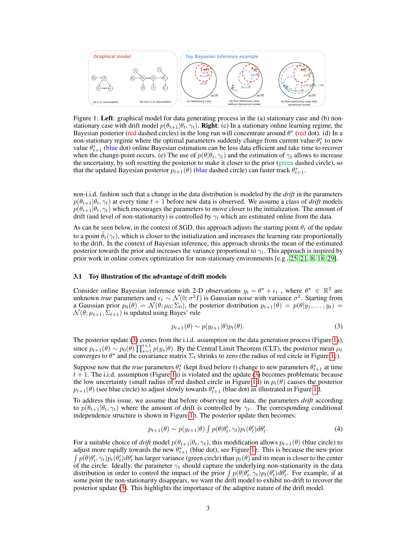
🔼 This table compares the computational cost and memory requirements for different methods discussed in the paper. The methods include standard SGD, Soft Reset with various configurations (drift parameter per layer or per parameter, with or without proximal updates), and Bayesian Soft Reset Proximal (also with variations). The cost is expressed in Big O notation, showing how it scales with relevant factors (S= cost of SGD backward pass, K= number of updates, M= number of Monte Carlo samples, P=number of parameters, L= number of layers). This helps to understand the computational trade-offs between the different approaches.
read the caption
Table 1: Comparison of methods, computational cost, and memory requirements
In-depth insights#
Soft Reset Mechanism#
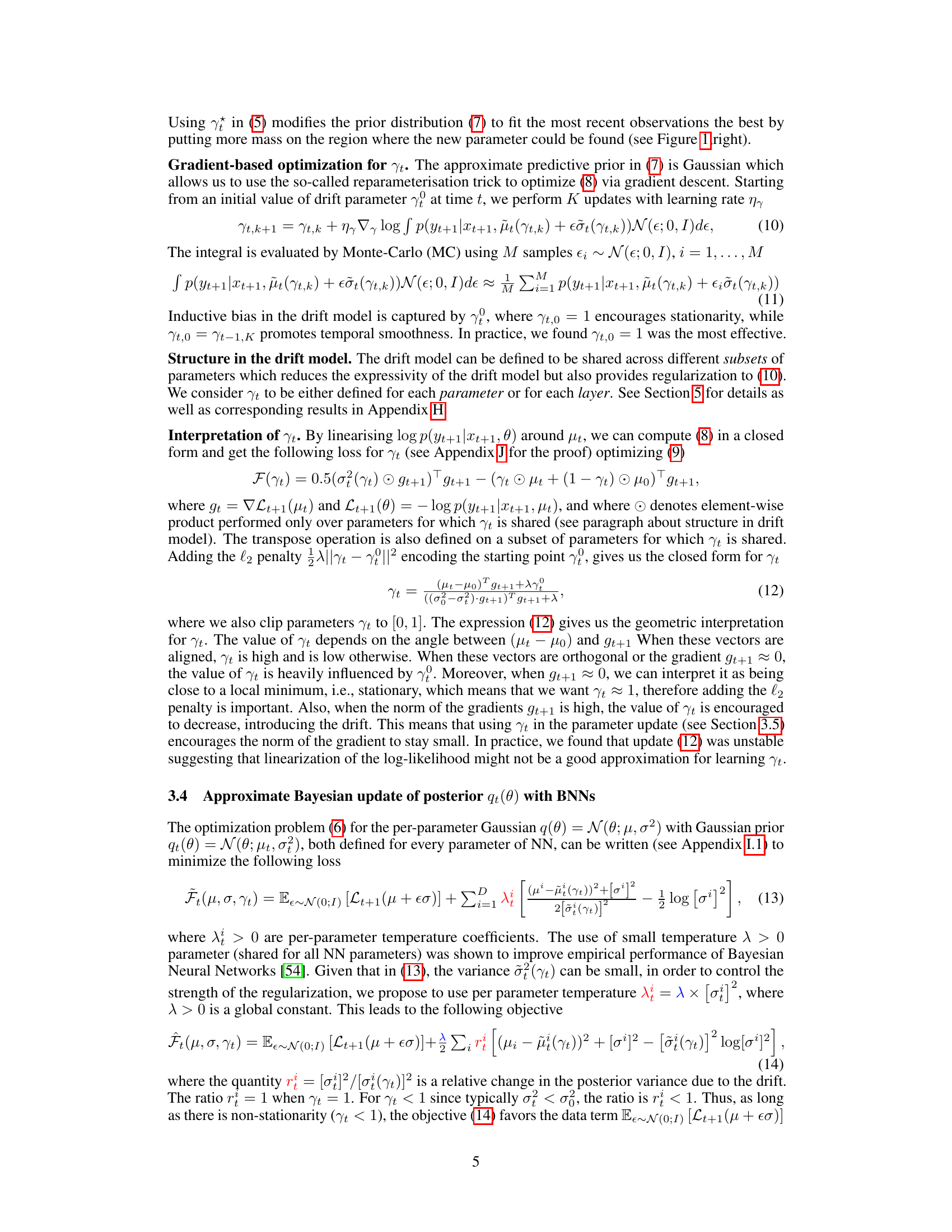
The proposed ‘Soft Reset Mechanism’ offers a novel approach to address the challenge of plasticity loss in neural networks trained on non-stationary data. Unlike traditional hard resets that abruptly discard learned parameters, this method introduces a soft, gradual shift of network parameters towards their initial values, controlled by a learned drift parameter. This drift, modeled as an Ornstein-Uhlenbeck process, dynamically adjusts the extent of the reset based on the perceived non-stationarity in the data. The mechanism effectively balances retaining valuable learned information with enabling adaptation to new data distributions. The adaptive nature of the soft reset, learning its parameters online, makes it particularly robust, and unlike methods requiring predefined schedules or heuristics for resets, this method automatically adapts to varying levels of non-stationarity. A key advantage is the implicit increase in effective learning rate that the soft reset engenders, facilitating quicker adaptation to shifts. Overall, the soft reset represents a significant advancement in continual learning, offering a more elegant and efficient solution to preserving plasticity and improving the robustness of neural networks in the face of non-stationary data.
Non-Stationary Learning#
Non-stationary learning tackles the challenge of training machine learning models on data whose underlying distribution changes over time. This is in contrast to traditional methods that assume a stationary distribution. The core issue is that models trained on a stationary distribution often fail to adapt effectively when the data distribution shifts. This paper addresses this by introducing a novel method that leverages an Ornstein-Uhlenbeck process to model the adaptation to non-stationarity, incorporating soft parameter resets. This approach contrasts sharply with hard resets, which discard valuable learned parameters. The adaptive drift parameter dynamically adjusts the influence of the initialization distribution, striking a balance between maintaining plasticity and adapting to the new data. The proposed methods are empirically evaluated in both supervised and reinforcement learning scenarios, demonstrating improved performance and the prevention of catastrophic forgetting. A key contribution is the online estimation of the drift parameter, allowing the model to dynamically adjust to different levels of non-stationarity. While the focus is on neural networks, the underlying principles of soft resets and adaptive drift parameters may find wider applications in various machine learning contexts dealing with evolving data distributions.
Drift Model Estimation#
Estimating the drift model is crucial for adapting to non-stationary data distributions. The authors propose using a predictive likelihood approach, selecting the prior distribution that best explains future data. This involves an approximate online variational inference method with Bayesian neural networks, updating the posterior distribution over NN parameters using the drift model. The drift is explicitly modeled using an Ornstein-Uhlenbeck process, with an adaptive drift parameter (γt) that controls the rate of movement toward the initialization distribution. The estimation process uses a gradient-based approach, optimizing predictive likelihood via gradient descent and the reparameterization trick. The adaptive nature of γt is key, allowing the model to react appropriately to different levels of non-stationarity. Online estimation is computationally efficient, crucial for real-time adaptation in non-stationary environments. The method is further enhanced by exploring shared parameters for improved stability and reducing model complexity.
Plasticity Benchmarks#
Plasticity benchmarks in the context of non-stationary learning for neural networks are crucial for evaluating a model’s ability to adapt to changing data distributions without catastrophic forgetting. These benchmarks typically involve a sequence of learning tasks, where the model is trained on each task consecutively. Performance is then measured on how well the model retains knowledge from previous tasks while learning new ones. Key aspects to consider are the type of task transitions (abrupt vs. gradual), the similarity between tasks, and the data efficiency of the approach. A good benchmark should reveal whether a model can retain learned knowledge and adapt quickly to new information, or if it suffers from catastrophic forgetting. It is vital to choose benchmarks that reflect the intended application scenarios, as the performance on a specific benchmark is not necessarily generalizable across all non-stationary settings. Analyzing performance across different plasticity benchmarks allows for a more robust assessment of a model’s generalization abilities and resilience to non-stationarity. The metrics chosen for evaluation, such as accuracy, loss, and forgetting rates, need to be carefully selected to highlight the specific aspects of plasticity being measured. This multifaceted approach is vital for the advancement of continual learning and the development of robust, adaptable neural network models.
RL Experiments#
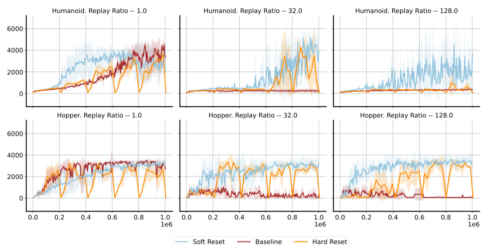
The RL experiments section would detail the application of the proposed soft parameter reset method within reinforcement learning (RL) environments. It would likely involve comparing the method against standard RL algorithms (like SAC or PPO) and other approaches that address plasticity loss. Key aspects would include the RL environments used (e.g., continuous control tasks in MuJoCo or similar), the performance metrics (such as cumulative reward or average episodic return), and the analysis of results considering factors like the level of off-policy data, task switching frequency, and the impact of hyperparameters. The experimental design should include sufficient control groups and rigorous statistical analysis to demonstrate the effectiveness of the proposed method. Success would be indicated by a significant improvement in performance compared to baselines, particularly in non-stationary or continual learning scenarios. The discussion would likely involve explaining the observed behaviors, examining the role of the drift parameter in adapting to non-stationarity and detailing the computational costs and scalability of the method. Failure to meet these criteria would necessitate further investigation into reasons for underperformance, such as limitations in the drift model or inherent challenges in applying soft resets to the chosen RL problem.
More visual insights#
More on figures

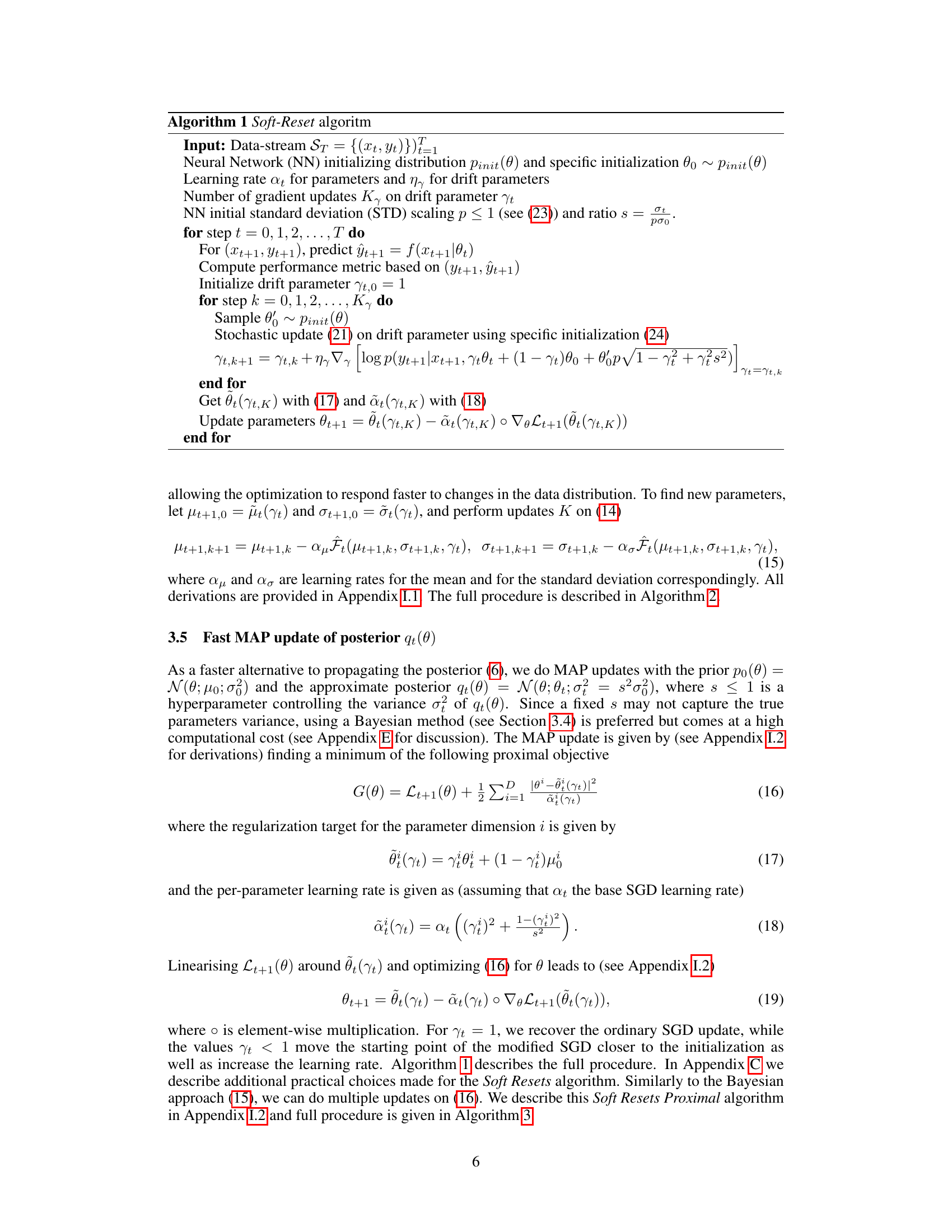
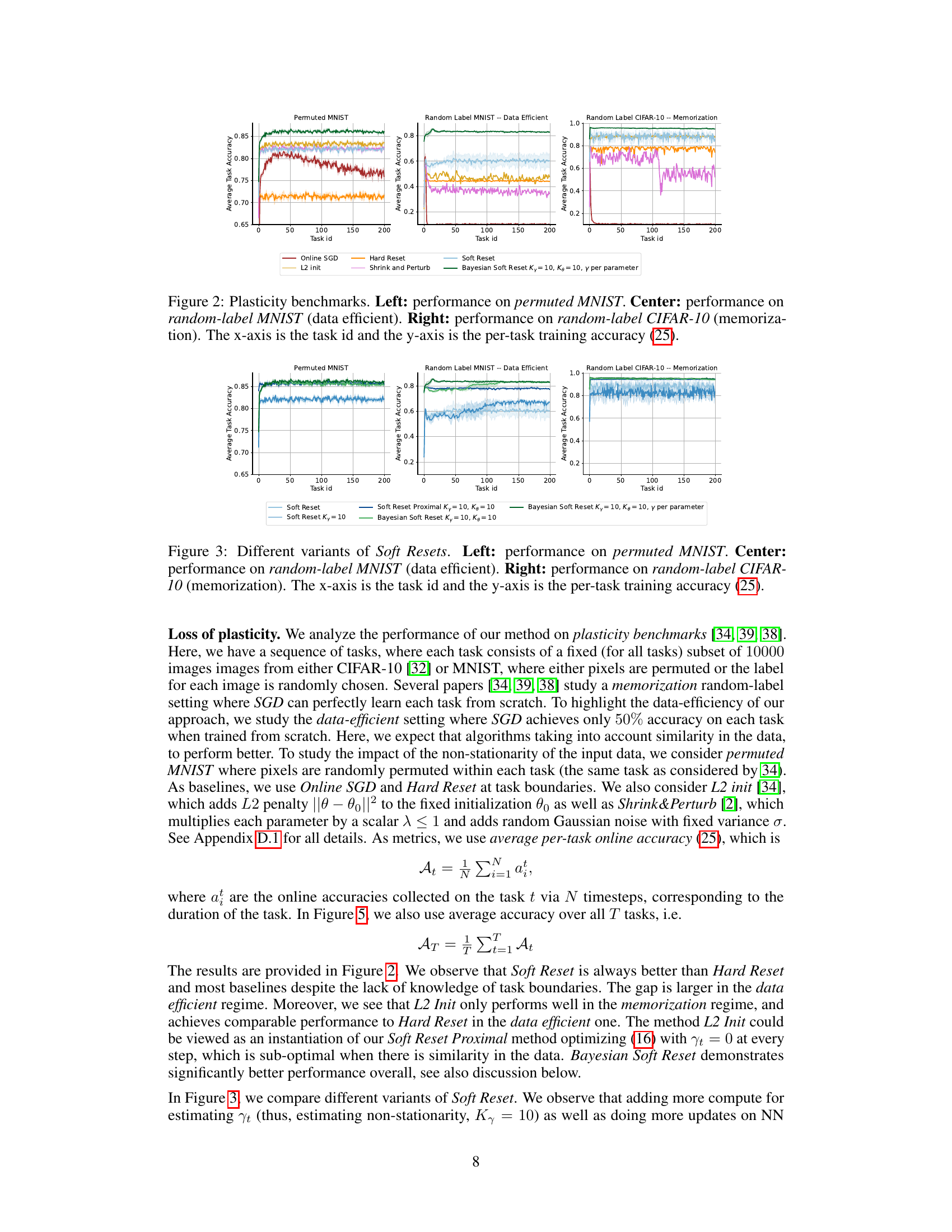
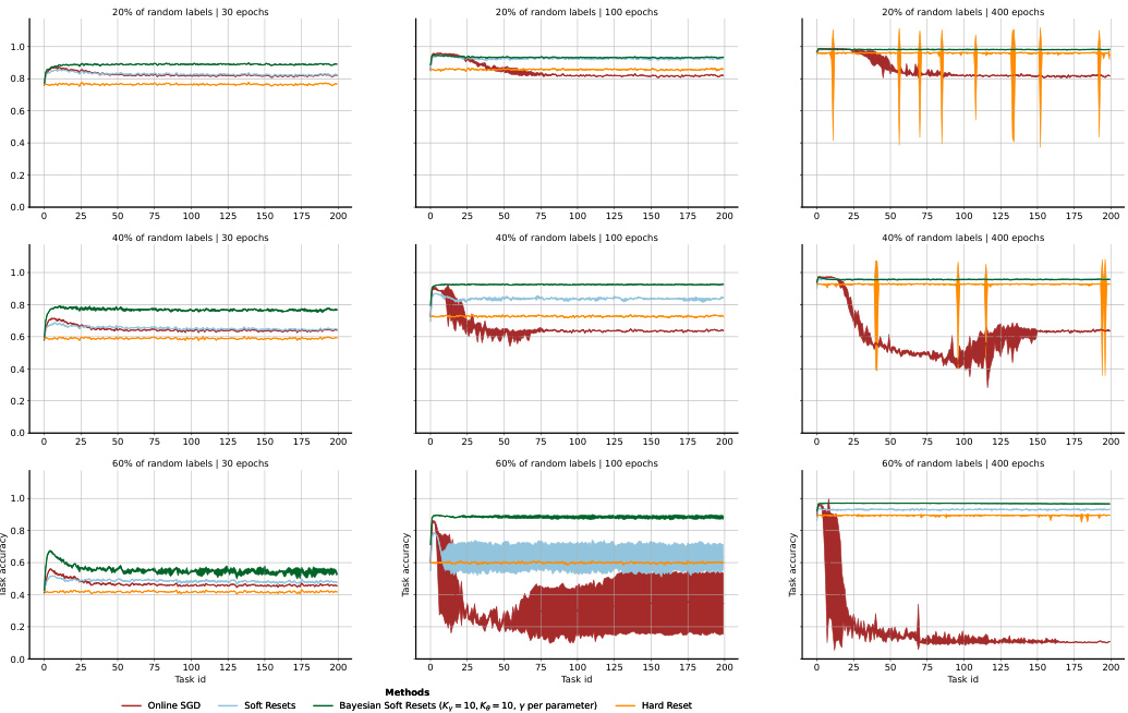
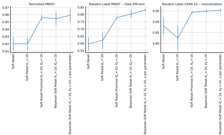
🔼 This figure compares the performance of different continual learning methods (Online SGD, L2 init, Hard Reset, Shrink and Perturb, Soft Reset, and Bayesian Soft Reset) across three different plasticity benchmarks: permuted MNIST, data-efficient random-label MNIST, and memorization random-label CIFAR-10. Each benchmark presents a unique challenge to continual learning, testing the ability of the methods to maintain performance across tasks. The x-axis represents the task ID, and the y-axis shows the per-task training accuracy. The results demonstrate that the Soft Reset and Bayesian Soft Reset methods significantly outperform the baselines in preserving performance across tasks, highlighting their ability to maintain plasticity.
read the caption
Figure 2: Plasticity benchmarks. Left: performance on permuted MNIST. Center: performance on random-label MNIST (data efficient). Right: performance on random-label CIFAR-10 (memorization). The x-axis is the task id and the y-axis is the per-task training accuracy (25).
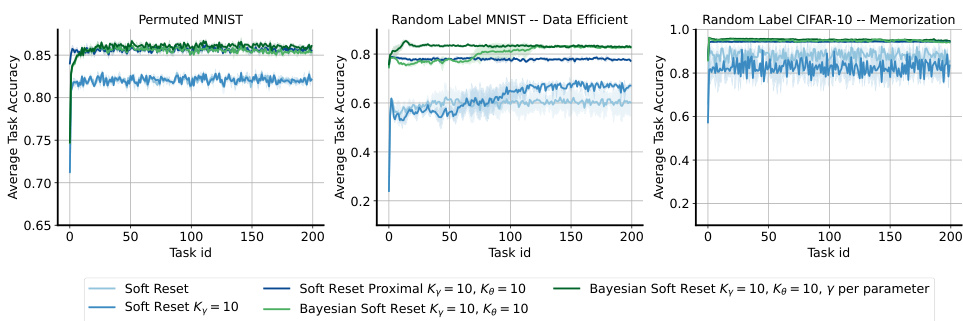
🔼 This figure compares the performance of different methods on three different plasticity benchmarks: permuted MNIST, data-efficient random-label MNIST, and memorization random-label CIFAR-10. The x-axis represents the task ID, and the y-axis shows the average per-task training accuracy. The results demonstrate the effectiveness of the proposed Soft Reset method in maintaining plasticity compared to other approaches, especially in the data-efficient and memorization settings.
read the caption
Figure 2: Plasticity benchmarks. Left: performance on permuted MNIST. Center: performance on random-label MNIST (data efficient). Right: performance on random-label CIFAR-10 (memorization). The x-axis is the task id and the y-axis is the per-task training accuracy (25).

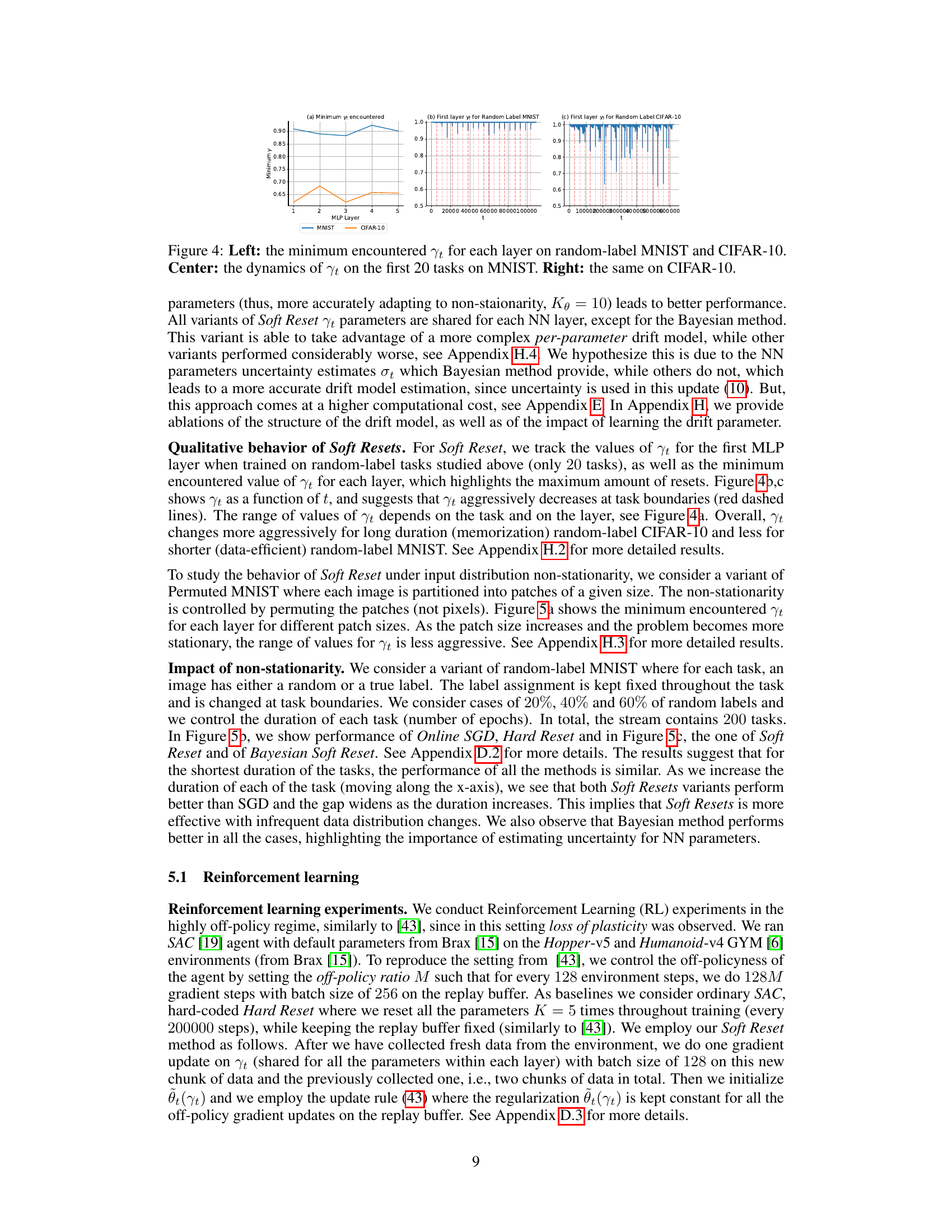
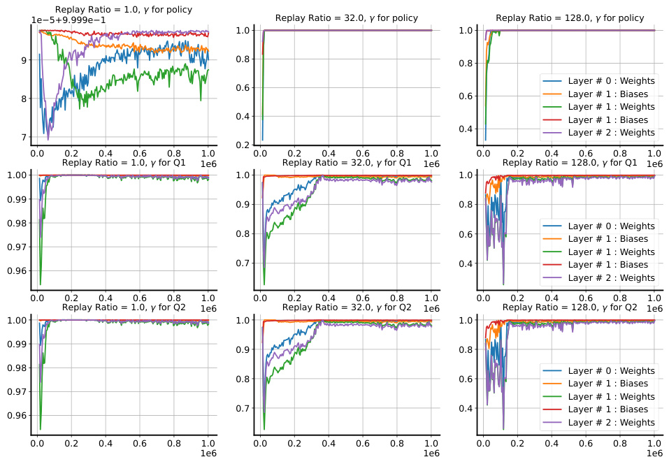
🔼 This figure visualizes the behavior of the learned drift parameter γt. The left panel shows the minimum value of γt encountered for each layer across all tasks, separately for MNIST and CIFAR-10 datasets. The center and right panels display the dynamics of γt for the first 20 tasks on MNIST and CIFAR-10, respectively, focusing on the first layer. The plots illustrate how γt changes over time and across different layers, providing insights into the adaptive nature of the soft reset mechanism in response to non-stationarity.
read the caption
Figure 4: Left: the minimum encountered γt for each layer on random-label MNIST and CIFAR-10. Center: the dynamics of γt on the first 20 tasks on MNIST. Right: the same on CIFAR-10.

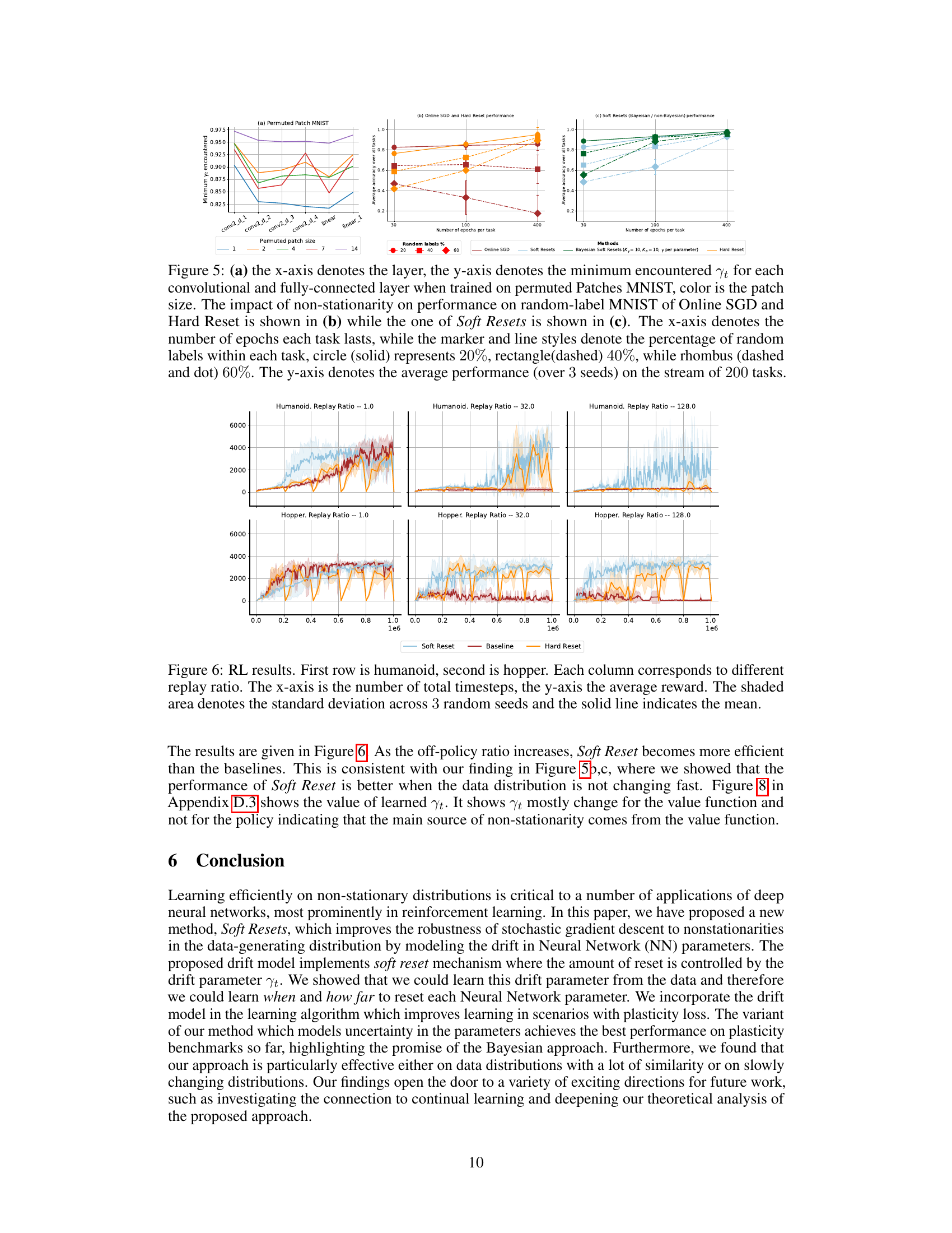
🔼 Figure 5 presents an analysis of non-stationarity effects. (a) shows how the minimum γt (minimum drift parameter value encountered) varies across layers in a permuted patch MNIST setup with different patch sizes. This reveals insights into how much the parameters drift across various network layers and with changing data non-stationarity levels (patch size). (b) plots the average task accuracy of Online SGD and Hard Reset across different numbers of epochs per task and varying random label percentages. It indicates how these methods handle varying levels of non-stationarity. (c) depicts the average task accuracy of Soft Reset methods (with and without Bayesian variants) across different epochs per task and random label percentages, showing their performance compared to baselines in non-stationary scenarios.
read the caption
Figure 5: (a) the x-axis denotes the layer, the y-axis denotes the minimum encountered γt for each convolutional and fully-connected layer when trained on permuted Patches MNIST, color is the patch size. The impact of non-stationarity on performance on random-label MNIST of Online SGD and Hard Reset is shown in (b) while the one of Soft Resets is shown in (c). The x-axis denotes the number of epochs each task lasts, while the marker and line styles denote the percentage of random labels within each task, circle (solid) represents 20%, rectangle(dashed) 40%, while rhombus (dashed and dot) 60%. The y-axis denotes the average performance (over 3 seeds) on the stream of 200 tasks.
🔼 This figure presents a comparison of different methods’ performance on three plasticity benchmarks: permuted MNIST, data-efficient random-label MNIST, and memorization random-label CIFAR-10. Each benchmark assesses the ability of a model to learn new tasks without forgetting previously learned ones, under different data conditions. The x-axis represents the task ID (indicating a sequence of tasks), while the y-axis shows the training accuracy achieved on each task. The results demonstrate the relative performance of several continual learning methods including Soft Reset and its variants, compared to existing approaches such as Online SGD, Hard Reset, L2-Init and Shrink & Perturb.
read the caption
Figure 2: Plasticity benchmarks. Left: performance on permuted MNIST. Center: performance on random-label MNIST (data efficient). Right: performance on random-label CIFAR-10 (memorization). The x-axis is the task id and the y-axis is the per-task training accuracy (25).
🔼 This figure presents the results of plasticity benchmarks on three different datasets: permuted MNIST, random-label MNIST (data-efficient), and random-label CIFAR-10 (memorization). The results compare the performance of several continual learning methods, including the proposed Soft Reset algorithm and baselines like Online SGD, L2-init, Hard Reset, and Shrink and Perturb. For each dataset, the x-axis represents the task ID, and the y-axis displays the per-task training accuracy. The plots show the ability of each method to maintain plasticity (the ability to learn new tasks without forgetting previously learned tasks) in different non-stationary scenarios.
read the caption
Figure 2: Plasticity benchmarks. Left: performance on permuted MNIST. Center: performance on random-label MNIST (data efficient). Right: performance on random-label CIFAR-10 (memorization). The x-axis is the task id and the y-axis is the per-task training accuracy (25).
🔼 This figure shows the results of plasticity benchmarks on three different datasets: permuted MNIST, random-label MNIST (data efficient), and random-label CIFAR-10 (memorization). Each subfigure represents a different dataset and compares the performance of several methods, including Soft Reset and several baselines. The x-axis represents the task ID, indicating the order in which the tasks were presented to the model, and the y-axis represents the per-task training accuracy.
read the caption
Figure 2: Plasticity benchmarks. Left: performance on permuted MNIST. Center: performance on random-label MNIST (data efficient). Right: performance on random-label CIFAR-10 (memorization). The x-axis is the task id and the y-axis is the per-task training accuracy (25).
🔼 This figure compares the performance of different continual learning methods on three benchmark tasks: permuted MNIST, data-efficient random-label MNIST, and memorization random-label CIFAR-10. Each task involves learning a new permutation of MNIST digits (left), a new random assignment of labels to MNIST digits (center - data efficient, meaning the model does not easily memorize), or learning to memorize new random labels assigned to CIFAR-10 images (right). The x-axis indicates the task ID, and the y-axis shows the training accuracy for each task. This illustrates the ability of the proposed Soft Reset method to maintain plasticity (the ability to learn new tasks without forgetting previous ones) compared to several baseline methods (Online SGD, L2 Init, Shrink and Perturb).
read the caption
Figure 2: Plasticity benchmarks. Left: performance on permuted MNIST. Center: performance on random-label MNIST (data efficient). Right: performance on random-label CIFAR-10 (memorization). The x-axis is the task id and the y-axis is the per-task training accuracy (25).

🔼 This figure compares the performance of different continual learning methods (Online SGD, L2 init, Hard Reset, Shrink and Perturb, Soft Reset, and Bayesian Soft Reset) across three different benchmarks: permuted MNIST, data-efficient random-label MNIST, and memorization random-label CIFAR-10. Each benchmark presents a unique challenge for continual learning, testing the algorithms’ ability to retain previous knowledge while adapting to new tasks. The x-axis represents the task ID, indicating the sequence of tasks, while the y-axis shows the per-task accuracy. The results illustrate the effectiveness of the Soft Reset methods, particularly the Bayesian variant, in preserving plasticity and maintaining high accuracy across the tasks compared to standard continual learning algorithms.
read the caption
Figure 2: Plasticity benchmarks. Left: performance on permuted MNIST. Center: performance on random-label MNIST (data efficient). Right: performance on random-label CIFAR-10 (memorization). The x-axis is the task id and the y-axis is the per-task training accuracy (25).

🔼 This figure displays the results of plasticity benchmarks on three different datasets: permuted MNIST, random-label MNIST (data-efficient), and random-label CIFAR-10 (memorization). Each subfigure shows the per-task training accuracy plotted against the task ID. The results compare the performance of Soft Reset and Bayesian Soft Reset against several baseline methods (Online SGD, L2 Init, Shrink and Perturb, and Hard Reset), demonstrating the effectiveness of the proposed Soft Reset approaches in maintaining plasticity and preventing catastrophic forgetting.
read the caption
Figure 2: Plasticity benchmarks. Left: performance on permuted MNIST. Center: performance on random-label MNIST (data efficient). Right: performance on random-label CIFAR-10 (memorization). The x-axis is the task id and the y-axis is the per-task training accuracy (25).

🔼 This figure compares the performance of different continual learning methods on three benchmark tasks. The tasks assess the ability of the models to maintain plasticity (the ability to learn new tasks without forgetting previously learned ones) under different levels of non-stationarity. The x-axis shows the task ID, and the y-axis represents the accuracy achieved on each task. The left panel shows permuted MNIST, where the pixels of the images are randomly permuted for each task. The center panel shows random-label MNIST (data-efficient), where random labels are assigned to MNIST images. The right panel shows random-label CIFAR-10 (memorization), a more challenging task. The results demonstrate that the proposed Soft Reset method achieves better performance compared to standard online SGD and other baselines (L2-init, Hard Reset, Shrink and Perturb) across all three tasks.
read the caption
Figure 2: Plasticity benchmarks. Left: performance on permuted MNIST. Center: performance on random-label MNIST (data efficient). Right: performance on random-label CIFAR-10 (memorization). The x-axis is the task id and the y-axis is the per-task training accuracy (25).

🔼 This figure compares the performance of different continual learning methods on three benchmark tasks: permuted MNIST, data-efficient random label MNIST, and memorization random label CIFAR-10. The x-axis represents the task ID, indicating the sequence of learning tasks. The y-axis shows the per-task training accuracy, providing a measure of how well each method maintains plasticity and avoids catastrophic forgetting as new tasks are introduced. The results demonstrate the effectiveness of the proposed Soft Reset method in handling non-stationary data distributions, particularly when compared to traditional methods like Online SGD, L2-Init, Shrink and Perturb, and Hard Reset.
read the caption
Figure 2: Plasticity benchmarks. Left: performance on permuted MNIST. Center: performance on random-label MNIST (data efficient). Right: performance on random-label CIFAR-10 (memorization). The x-axis is the task id and the y-axis is the per-task training accuracy (25).

🔼 This figure compares the performance of different continual learning methods on three benchmark datasets: permuted MNIST, data-efficient random-label MNIST, and memorization random-label CIFAR-10. Each dataset presents a different challenge in terms of non-stationarity. The x-axis represents the task ID, indicating the progression through a sequence of learning tasks. The y-axis represents the per-task training accuracy, measuring the model’s ability to learn and retain knowledge across tasks. The figure shows that Soft Reset consistently outperforms other methods across all three benchmarks, highlighting its effectiveness in maintaining plasticity (the ability to learn new tasks without forgetting previously learned ones).
read the caption
Figure 2: Plasticity benchmarks. Left: performance on permuted MNIST. Center: performance on random-label MNIST (data efficient). Right: performance on random-label CIFAR-10 (memorization). The x-axis is the task id and the y-axis is the per-task training accuracy (25).

🔼 This figure compares the performance of different continual learning methods (Online SGD, L2 init, Hard Reset, Shrink and Perturb, Soft Reset, and Bayesian Soft Reset) on three different plasticity benchmarks: permuted MNIST, data-efficient random-label MNIST, and memorization random-label CIFAR-10. The x-axis represents the task ID, and the y-axis shows the per-task training accuracy. The results demonstrate the effectiveness of Soft Reset and Bayesian Soft Reset in maintaining plasticity, especially compared to methods that employ hard resets.
read the caption
Figure 2: Plasticity benchmarks. Left: performance on permuted MNIST. Center: performance on random-label MNIST (data efficient). Right: performance on random-label CIFAR-10 (memorization). The x-axis is the task id and the y-axis is the per-task training accuracy (25).

🔼 This figure compares the performance of different variants of Soft Reset on data-efficient random-label MNIST. The left panel shows Soft Reset with a constant learning rate, while the right panel shows Soft Reset with a higher learning rate at task switches (when γ < 1). The results demonstrate the impact of increasing the learning rate at the task boundaries for improving the learning efficiency and plasticity. The plot shows that Soft Reset with a higher learning rate outperforms the baselines, and it shows the impact of different values of gamma (γ) on plasticity in this setting.
read the caption
Figure 16: Perfect soft-resets on data-efficient random-label MNIST. Left, Soft Reset method does not use higher learning rate when γ < 1. Right, Soft Reset increases the learning rate when γ < 1, see (18). The x-axis represents task id, whereas the y-axis is the average training accuracy on the task.

🔼 This figure shows the results of plasticity benchmarks on three different datasets: permuted MNIST, random-label MNIST (data efficient), and random-label CIFAR-10 (memorization). Each subfigure represents a different dataset and compares the performance of several methods, including Soft Reset and baselines such as Online SGD, L2-init, Hard Reset, and Shrink and Perturb. The x-axis represents the task ID, indicating the sequence of tasks in the continual learning setting. The y-axis shows the per-task training accuracy, which is a measure of how well each method performs on each individual task. The figure demonstrates the Soft Reset method’s ability to maintain plasticity (the ability to learn new tasks without forgetting previously learned tasks) across the different datasets and task sequences compared to the baselines.
read the caption
Figure 2: Plasticity benchmarks. Left: performance on permuted MNIST. Center: performance on random-label MNIST (data efficient). Right: performance on random-label CIFAR-10 (memorization). The x-axis is the task id and the y-axis is the per-task training accuracy (25).

🔼 This figure compares the performance of different methods (Online SGD, L2 init, Hard Reset, Shrink and Perturb, Soft Reset, and Bayesian Soft Reset) on three different plasticity benchmarks: permuted MNIST, data-efficient random-label MNIST, and memorization random-label CIFAR-10. The x-axis represents the task ID (a sequence of learning tasks), and the y-axis shows the per-task training accuracy. The results demonstrate the effectiveness of the proposed Soft Reset method in maintaining plasticity, especially when compared to traditional methods like Online SGD and Hard Reset.
read the caption
Figure 2: Plasticity benchmarks. Left: performance on permuted MNIST. Center: performance on random-label MNIST (data efficient). Right: performance on random-label CIFAR-10 (memorization). The x-axis is the task id and the y-axis is the per-task training accuracy (25).

🔼 This figure compares the performance of different methods (Online SGD, L2 Init, Hard Reset, Shrink and Perturb, Soft Reset, and Bayesian Soft Reset) on three different plasticity benchmarks: permuted MNIST, data-efficient random-label MNIST, and memorization random-label CIFAR-10. Each benchmark presents a unique challenge in continual learning due to varying degrees of data distribution shift and task similarity. The x-axis represents the task ID, while the y-axis shows the per-task training accuracy. The results demonstrate that the proposed Soft Reset methods, especially the Bayesian Soft Reset, significantly improve performance compared to standard methods on these challenging benchmarks.
read the caption
Figure 2: Plasticity benchmarks. Left: performance on permuted MNIST. Center: performance on random-label MNIST (data efficient). Right: performance on random-label CIFAR-10 (memorization). The x-axis is the task id and the y-axis is the per-task training accuracy (25).

🔼 This figure displays the results of plasticity benchmarks on three different datasets: permuted MNIST, random-label MNIST (data-efficient setting), and random-label CIFAR-10 (memorization setting). The x-axis represents the task ID, indicating the sequence of tasks. The y-axis shows the per-task training accuracy. Several methods, including Online SGD, L2 Init, Shrink and Perturb, Hard Reset, Soft Reset, and Bayesian Soft Reset, are compared to evaluate their ability to maintain plasticity (the ability to learn new tasks without forgetting previous ones) under non-stationary conditions. Each dataset and setting presents a different challenge, and the results highlight the relative performance of each method.
read the caption
Figure 2: Plasticity benchmarks. Left: performance on permuted MNIST. Center: performance on random-label MNIST (data efficient). Right: performance on random-label CIFAR-10 (memorization). The x-axis is the task id and the y-axis is the per-task training accuracy (25).

🔼 This figure compares the performance of different continual learning methods (Online SGD, L2 init, Hard Reset, Shrink and Perturb, Soft Reset, and Bayesian Soft Reset) on three different plasticity benchmarks. Each benchmark involves a sequence of learning tasks where the data distribution changes between tasks. The left panel shows the performance on the permuted MNIST dataset, the center panel shows performance on a data-efficient version of random-label MNIST, and the right panel shows performance on a memorization version of random-label CIFAR-10. The x-axis shows the task ID, indicating the order in which tasks were presented. The y-axis shows the per-task training accuracy, representing the model’s performance on each task. The figure demonstrates the effectiveness of the Soft Reset methods in maintaining plasticity across multiple tasks, outperforming baseline methods in preventing catastrophic forgetting.
read the caption
Figure 2: Plasticity benchmarks. Left: performance on permuted MNIST. Center: performance on random-label MNIST (data efficient). Right: performance on random-label CIFAR-10 (memorization). The x-axis is the task id and the y-axis is the per-task training accuracy (25).

🔼 This figure illustrates the data generating process in both stationary and non-stationary scenarios, highlighting the benefits of the proposed drift model in handling non-stationarity. The left side shows the graphical models for both cases, comparing i.i.d and non-i.i.d assumptions. The right side provides a visual representation of Bayesian posterior updates under these scenarios and how the drift model improves efficiency and speed in adapting to changes.
read the caption
Figure 1: Left: graphical model for data generating process in the (a) stationary case and (b) non-stationary case with drift model p(θt+1|θt, Yt). Right: (c) In a stationary online learning regime, the Bayesian posterior (red dashed circles) in the long run will concentrate around θ* (red dot). (d) In a non-stationary regime where the optimal parameters suddenly change from current value θ to new value θt+1 (blue dot) online Bayesian estimation can be less data efficient and take time to recover when the change-point occurs. (e) The use of p(θ|θt, γt) and the estimation of γt allows to increase the uncertainty, by soft resetting the posterior to make it closer to the prior (green dashed circle), so that the updated Bayesian posterior pt+1(θ) (blue dashed circle) can faster track θt+1.
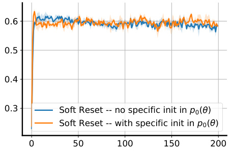
🔼 This figure shows the impact of using a specific initialization (θ0) in the prior distribution (p0(θ)) for the Soft Reset algorithm. Two variants of Soft Reset are compared: one where the prior’s mean is set to a specific initialization (θ0), and another where the prior’s mean is set to 0. The y-axis shows the average task accuracy across multiple tasks, with error bars representing the standard deviation across 3 random seeds. The results show similar performance for both variants, suggesting that the choice of initialization in the prior may not be as crucial for the Soft Reset algorithm’s performance.
read the caption
Figure 23: Impact of specific initialization θ0 as a mean of po(θ) in Soft Resets. The x-axis represents task id. The y-axis represents the average task accuracy with standard deviation computed over 3 random seeds. The task is random label MNIST - data efficient.

🔼 This figure shows a comparison of different SGD approaches for tracking a non-stationary mean in a toy problem. The true mean switches between -2 and 2 every 50 timesteps. The figure compares standard SGD with two different learning rates (0.05 and 0.15) against SGD methods that include parameter resets at the switch points with different reset learning rates. The results illustrate how parameter resets with appropriate learning rate scheduling can significantly improve adaptation to non-stationarity, allowing for faster convergence to the new mean compared to standard SGD.
read the caption
Figure 24: Non-stationary mean tracking with SGD.
More on tables

🔼 This table compares the computational cost and memory requirements of different methods discussed in the paper, including SGD, Soft Resets with various configurations (gamma per layer, gamma per parameter, with and without proximal updates), and Bayesian Soft Reset Proximal. The cost is expressed in big O notation, reflecting the dominant terms as the problem size increases. The memory requirements describe the space complexity of each method.
read the caption
Table 1: Comparison of methods, computational cost, and memory requirements

🔼 This table compares the computational cost and memory requirements of different methods for non-stationary learning. The methods include standard SGD, Soft Resets with different parameterizations (per layer and per parameter), Soft Resets with proximal updates (with different iterations), and Bayesian Soft Reset with proximal updates. The computational cost is given in Big O notation, considering the number of parameters (P), layers (L), SGD backward passes (S), Monte Carlo samples for drift parameter (My), Monte Carlo samples for parameter updates (Me), number of updates for drift parameters (Ky), and number of NN parameter updates (Ke). The memory requirements are also expressed in Big O notation.
read the caption
Table 1: Comparison of methods, computational cost, and memory requirements
Full paper#

