TL;DR#
Many generative models rely on conditional paths to transform data distributions, often assuming Euclidean geometry. This can lead to poor interpolations for complex, non-Euclidean data. Straight interpolations might not capture the data’s underlying dynamics and may fail to accurately represent the true trajectory when inferring systems’ dynamics from limited data. This is particularly problematic for applications with curved data manifolds, such as trajectory inference in single-cell RNA sequencing.
The proposed METRIC FLOW MATCHING (MFM) tackles this issue. It learns interpolants as approximate geodesics on a data-induced Riemannian manifold by minimizing the kinetic energy. MFM is simulation-free and employs general metrics, independent of specific tasks. Experiments across LiDAR navigation, unpaired image translation, and single-cell dynamics demonstrate MFM’s superiority over Euclidean baselines, achieving state-of-the-art results in single-cell trajectory prediction. The results show the efficiency of the proposed method in generating more meaningful interpolations that respect the data manifold.
Key Takeaways#
Why does it matter?#
This paper is crucial for researchers working on generative models and trajectory inference. It provides a novel framework that significantly improves interpolation quality by accounting for the underlying data manifold’s geometry. This is especially important for complex data where Euclidean assumptions fail, such as single-cell analysis, and opens avenues for developing more accurate and meaningful generative models for various scientific domains.
Visual Insights#

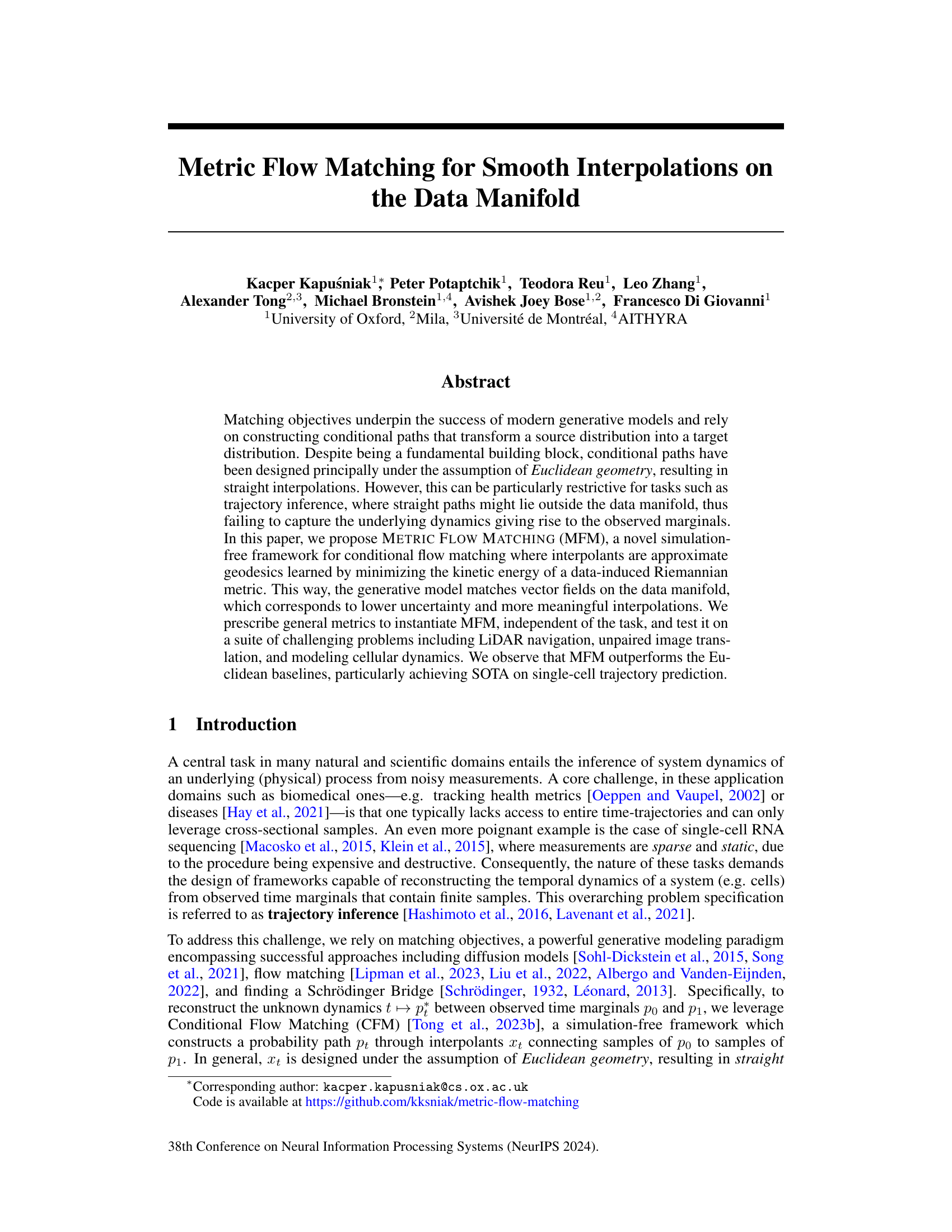
🔼 This figure illustrates the core idea of the paper. On the left, a comparison is shown between straight interpolations (as used in Conditional Flow Matching, CFM) and interpolations that follow a data-dependent Riemannian metric (Metric Flow Matching, MFM). The latter method keeps the interpolations closer to the data manifold. The right side shows the resulting probability densities at t = 0.5 from each method. MFM’s density is more concentrated and closer to the data manifold, indicating a more meaningful reconstruction.
read the caption
Figure 1: In orange and violet the source and target distributions. On the left, straight interpolations vs interpolations following a data-dependent Riemannian metric. On the right, densities of reconstructed marginals at time t = ½, using Conditional Flow Matching and METRIC FLOW MATCHING (MFM), respectively. MFM provides a more meaningful reconstruction supported on the data manifold.
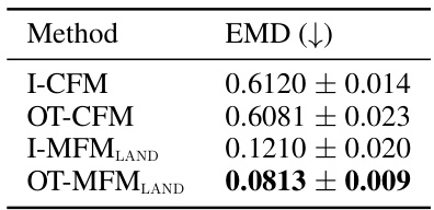
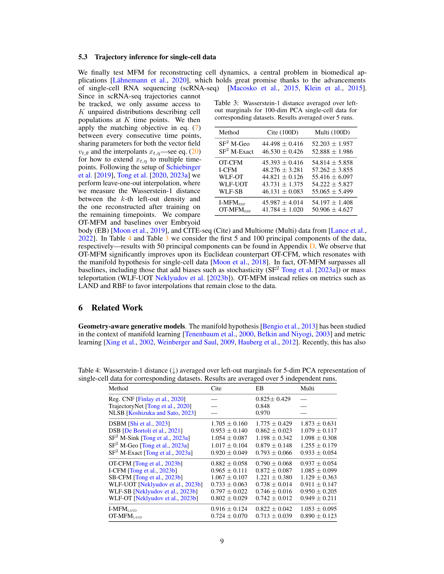
🔼 This table presents the Wasserstein distance (EMD) between the reconstructed marginal distribution at time t=1/2 and the ground truth distribution for different methods. Lower EMD values indicate better reconstruction accuracy. The methods compared are I-CFM (Independent Conditional Flow Matching), OT-CFM (Optimal Transport Conditional Flow Matching), I-MFMLAND (Independent Metric Flow Matching with LAND metric), and OT-MFMLAND (Optimal Transport Metric Flow Matching with LAND metric). The OT-MFMLAND method achieves the lowest EMD, demonstrating its superior performance in reconstructing the target distribution.
read the caption
Table 1: Wasserstein distance between reconstructed marginal at time 1/2 and ground-truth.
In-depth insights#
MFM: A New Approach#
The heading “MFM: A New Approach” suggests an innovative method (MFM) is introduced within the research paper. A thoughtful analysis would delve into what problem MFM solves, its core methodology, and its advantages over existing techniques. The paragraph should highlight the novelty of MFM, potentially mentioning if it’s a novel algorithm, model architecture, or a framework. Crucially, the summary should touch upon the practical applications of MFM, emphasizing its potential impact and its performance relative to benchmarks. Key aspects to consider include efficiency, scalability, and the extent to which MFM addresses limitations of prior methods. Finally, a thorough exploration would also acknowledge any limitations of MFM and suggest potential areas for future research.
Riemannian Geometry#
Riemannian geometry provides a powerful framework for extending concepts of Euclidean geometry to curved spaces. This is crucial when dealing with data that naturally resides on a manifold, rather than in a flat Euclidean space. In the context of the research paper, the use of Riemannian geometry allows the model to handle the inherent nonlinearity of data, enabling a more faithful representation of the underlying dynamics. The key idea is that by defining a Riemannian metric (an inner product on each tangent space of the manifold), the model can calculate distances and curves (geodesics) that conform to the data’s intrinsic geometry, instead of imposing artificial straight lines in Euclidean space which might ignore the manifold structure. This results in smoother and more meaningful interpolations, leading to better performance in trajectory inference and other applications.
MFM vs. CFM#
The core difference between MFM and CFM lies in how they handle interpolations within the data manifold. CFM, operating under the Euclidean assumption, generates straight-line interpolations, which often deviate from the underlying data’s complex geometry, particularly in non-Euclidean spaces. This limitation can lead to less meaningful and less accurate results, especially when the data’s intrinsic structure is non-linear. In contrast, MFM leverages a data-dependent Riemannian metric, which allows interpolations to follow geodesics, the shortest paths within the curved data manifold. By minimizing the kinetic energy induced by this metric, MFM learns interpolants that closely adhere to the data’s shape, thus resulting in smoother and more accurate estimations of the underlying process. MFM’s approach addresses CFM’s shortcomings by incorporating the manifold hypothesis, acknowledging that real-world data often resides on low-dimensional manifolds embedded in high-dimensional ambient spaces. As a result, MFM consistently yields better results in trajectory inference and similar tasks, particularly in single-cell trajectory prediction.
Single-Cell Dynamics#
Analyzing single-cell dynamics is crucial for understanding fundamental biological processes. Trajectory inference, a key aspect of this analysis, aims to reconstruct the temporal evolution of cellular states from noisy, sparse measurements. Traditional methods often struggle with the high dimensionality and nonlinearity inherent in single-cell data, leading to inaccurate or incomplete trajectory reconstructions. The manifold hypothesis, which posits that biological data resides on a low-dimensional manifold embedded in a high-dimensional space, provides a valuable framework. By leveraging this hypothesis, sophisticated methods, such as those using optimal transport or Riemannian geometry, can significantly improve trajectory inference accuracy. These methods consider the underlying geometry of the data, capturing the complex relationships between different cellular states. This refined approach yields more biologically meaningful interpolations and better captures the dynamic processes driving cellular changes. METRIC FLOW MATCHING (MFM) is an example method that utilizes a data-dependent Riemannian metric to achieve this improvement. The success of MFM in outperforming euclidean baselines on single cell trajectory prediction demonstrates the considerable potential of this data-informed geometric approach for extracting valuable biological insights from single-cell data.
Future Work#
Future research directions stemming from this work could explore several promising avenues. Extending MFM to handle more complex data structures and manifolds beyond Euclidean space is crucial. This might involve developing new methods for defining Riemannian metrics on non-Euclidean spaces or using alternative manifold learning techniques. Additionally, investigating the theoretical properties of MFM in the context of different metrics and coupling methods would provide a deeper understanding of its strengths and limitations. The development of more efficient algorithms for computing geodesics remains a significant challenge and warrants further investigation, especially for high-dimensional datasets. Finally, applying MFM to a wider range of applications and problem domains, such as time series forecasting, molecular dynamics simulation, and other scientific fields, is a promising area for future work. Further exploration into the interplay between MFM and existing trajectory inference methods is essential, aiming to create potentially more powerful and robust approaches.
More visual insights#
More on figures
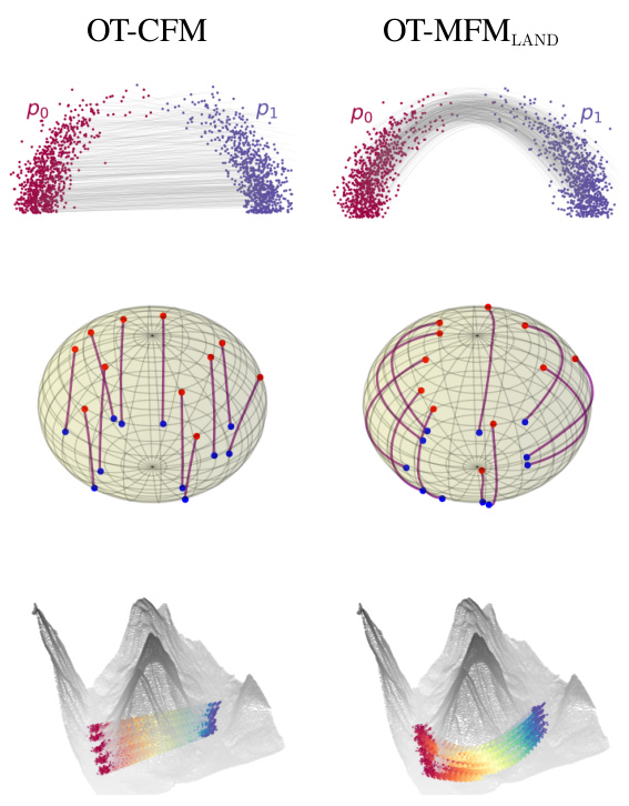
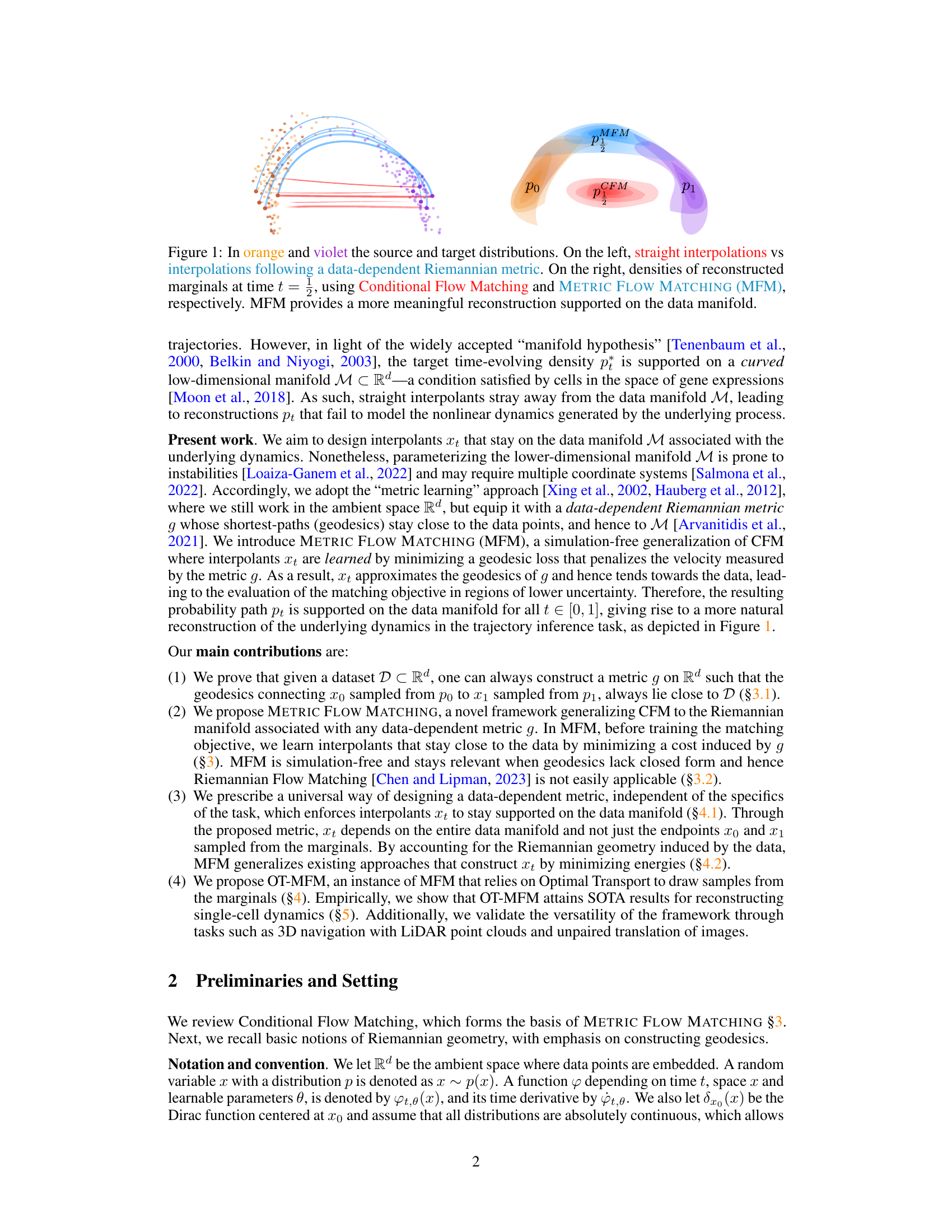
🔼 This figure illustrates the core idea of the paper: using a Riemannian metric to learn smooth interpolations on the data manifold. The left panel compares straight interpolations (CFM) with interpolations that follow a data-dependent Riemannian metric (MFM). The right panel shows the reconstructed probability densities at t=0.5 for both methods, highlighting that MFM yields more realistic results by staying on the data manifold.
read the caption
Figure 1: In orange and violet the source and target distributions. On the left, straight interpolations vs interpolations following a data-dependent Riemannian metric. On the right, densities of reconstructed marginals at time t = ½, using Conditional Flow Matching and METRIC FLOW MATCHING (MFM), respectively. MFM provides a more meaningful reconstruction supported on the data manifold.

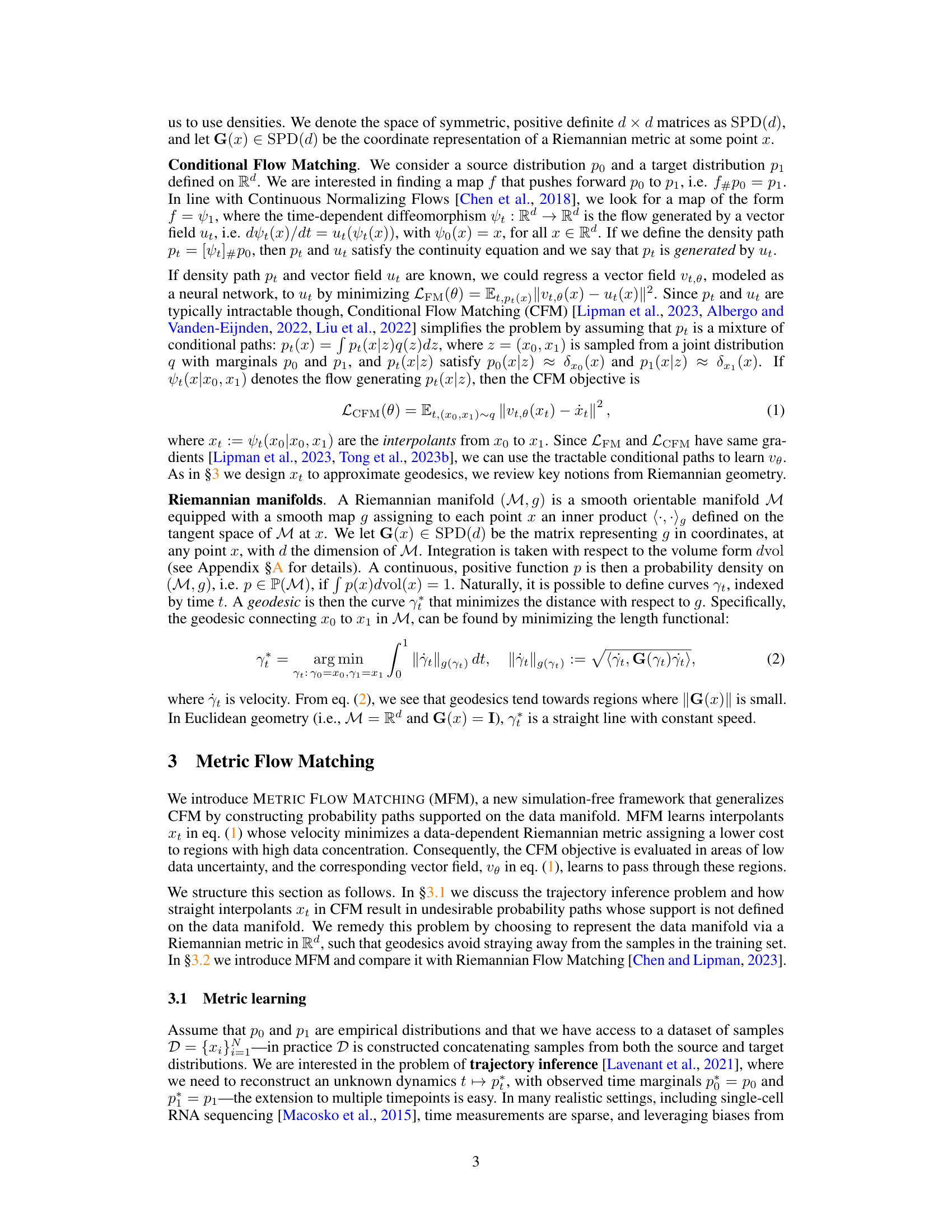
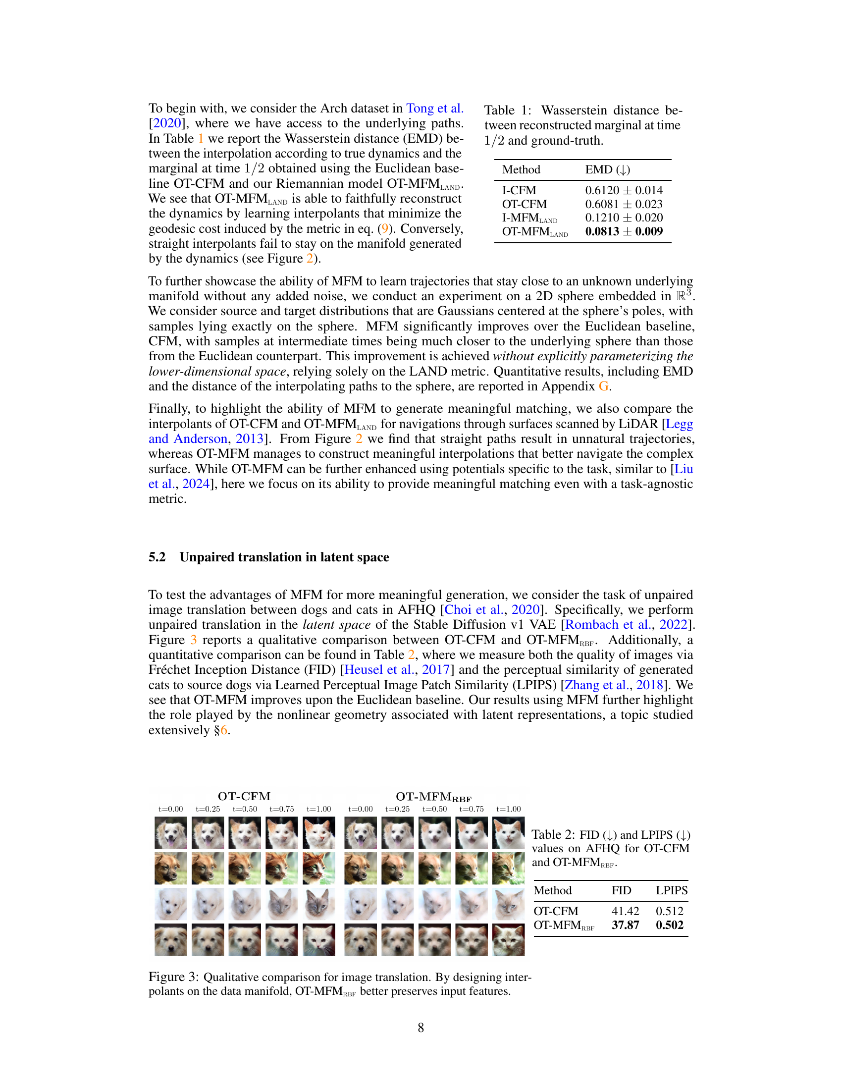
🔼 This figure compares the results of unpaired image translation between dogs and cats using two different methods: OT-CFM and OT-MFMRBF. OT-CFM uses straight interpolations in the latent space, while OT-MFMRBF uses interpolations that follow the data manifold. The images show that OT-MFMRBF better preserves the features of the source images (dogs) during the translation process, resulting in more realistic and coherent cat images. This demonstrates the effectiveness of the proposed metric flow matching method in generating higher-quality results for image generation tasks. Each column represents an intermediate time step in the translation process, from the source image (dog) at t = 0.00 to the target image (cat) at t = 1.00.
read the caption
Figure 3: Qualitative comparison for image translation. By designing interpolants on the data manifold, OT-MFMRBF better preserves input features.
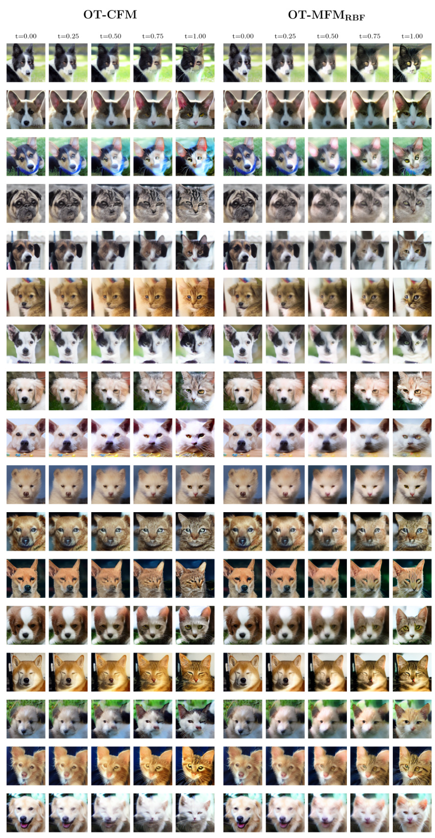
🔼 This figure shows a qualitative comparison of the image translation results between OT-CFM (left) and OT-MFMRBF (right). Both methods are applied to translate images of dogs into images of cats in the AFHQ dataset, using the latent space of the Stable Diffusion VAE. The images in the columns represent interpolated results at different points (t=0.00, t=0.25, t=0.50, t=0.75, t=1.00) along a path between the source (dog) and target (cat) distributions. The figure demonstrates that OT-MFMRBF, by incorporating the data manifold into the interpolation process, is better able to maintain the key features of the input image throughout the translation, resulting in more visually coherent and realistic-looking intermediate images compared to OT-CFM.
read the caption
Figure 3: Qualitative comparison for image translation. By designing interpolants on the data manifold, OT-MFMRBF better preserves input features.
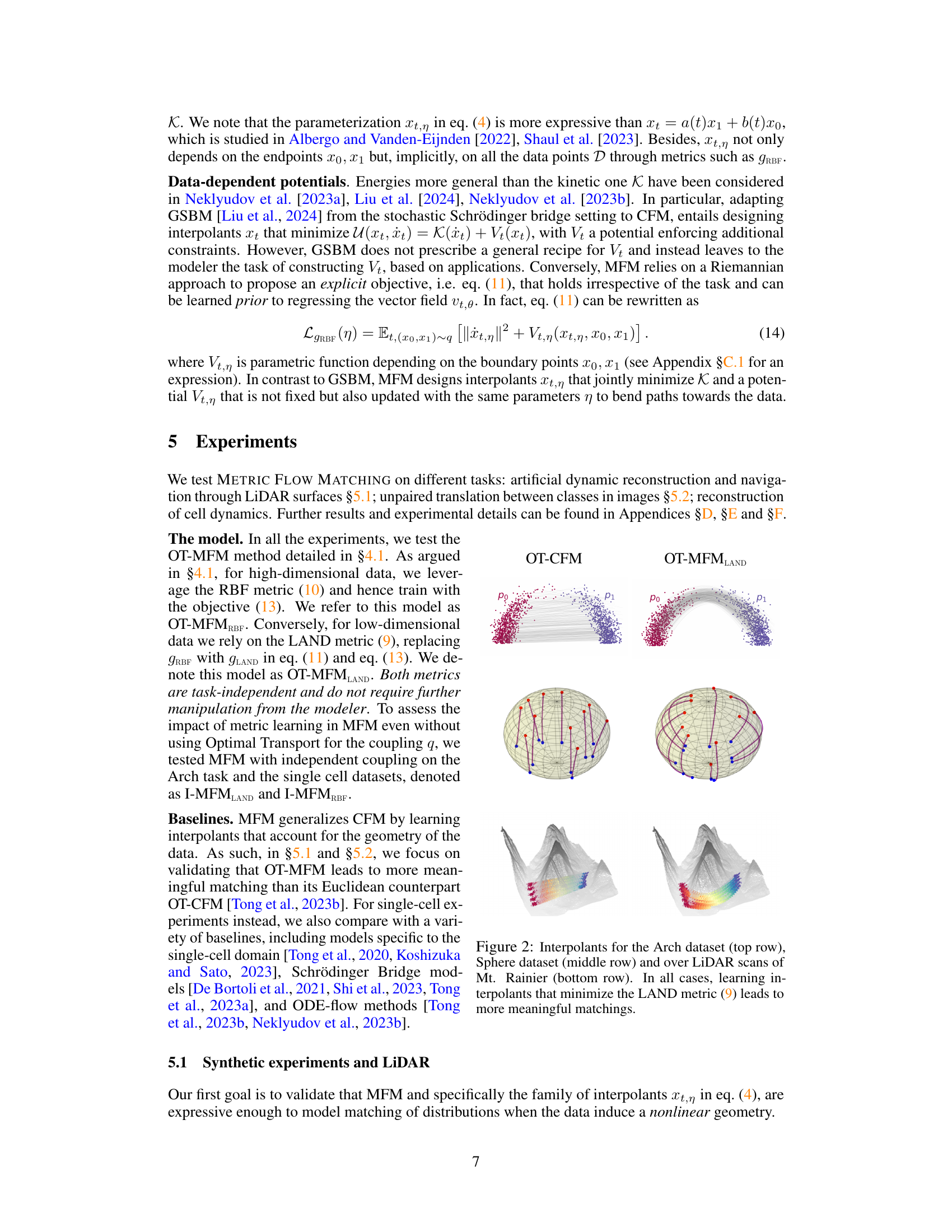
🔼 This figure illustrates the core idea of the paper. On the left, it compares straight-line interpolation (typical in Conditional Flow Matching or CFM) to interpolation along geodesics determined by a data-dependent Riemannian metric (using METRIC FLOW MATCHING or MFM). The right side shows the resulting probability densities at a specific time point (t=1/2) for both methods; MFM’s result better reflects the data manifold, representing improved interpolation.
read the caption
Figure 1: In orange and violet the source and target distributions. On the left, straight interpolations vs interpolations following a data-dependent Riemannian metric. On the right, densities of reconstructed marginals at time t = ½, using Conditional Flow Matching and METRIC FLOW MATCHING (MFM), respectively. MFM provides a more meaningful reconstruction supported on the data manifold.

🔼 This figure shows a comparison between Conditional Flow Matching (CFM) and Metric Flow Matching (MFM) methods for generating interpolations between two distributions. The left panel illustrates the difference between straight interpolations (CFM) and interpolations that follow a data-dependent Riemannian metric (MFM). The right panel shows the resulting density distributions at an intermediate time point, demonstrating that MFM generates more meaningful interpolations that lie within the data manifold.
read the caption
Figure 1: In orange and violet the source and target distributions. On the left, straight interpolations vs interpolations following a data-dependent Riemannian metric. On the right, densities of reconstructed marginals at time t = ½, using Conditional Flow Matching and METRIC FLOW MATCHING (MFM), respectively. MFM provides a more meaningful reconstruction supported on the data manifold.
More on tables
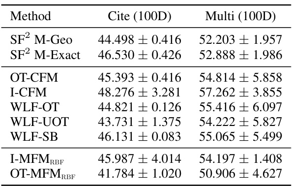
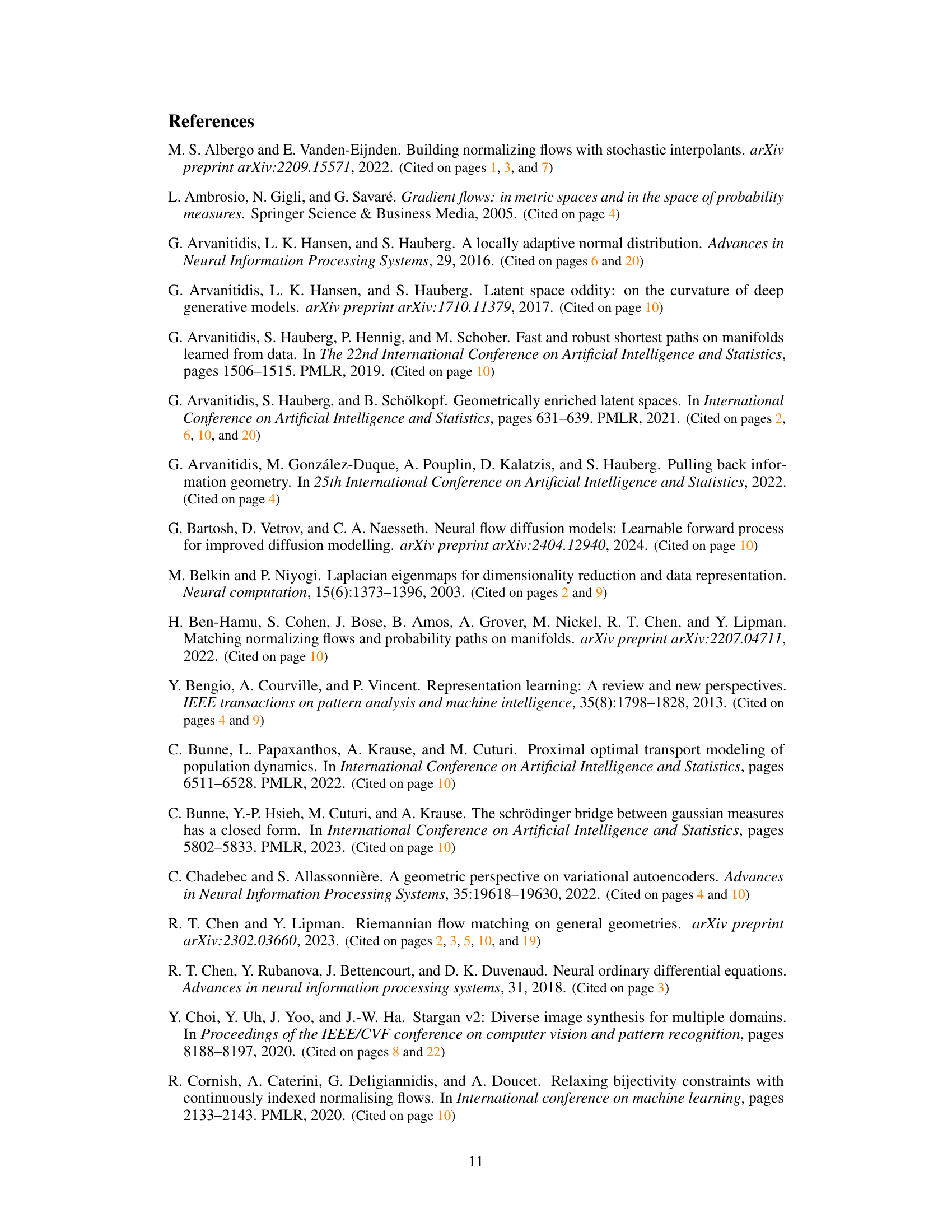
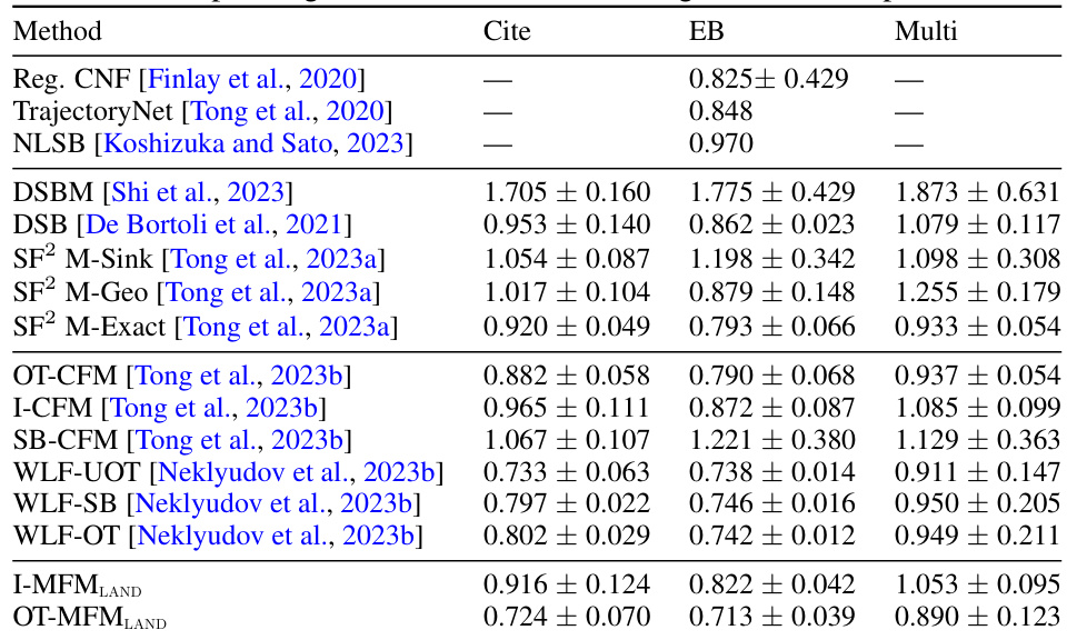
🔼 This table presents the Wasserstein-1 distance results for trajectory inference on single-cell data using 100 principal components. It compares the performance of various methods, including the proposed OT-MFM, against several baselines across three datasets: Cite, EB, and Multi. Lower values indicate better performance.
read the caption
Table 3: Wasserstein-1 distance averaged over left-out marginals for 100-dim PCA single-cell data for corresponding datasets. Results averaged over 5 runs.
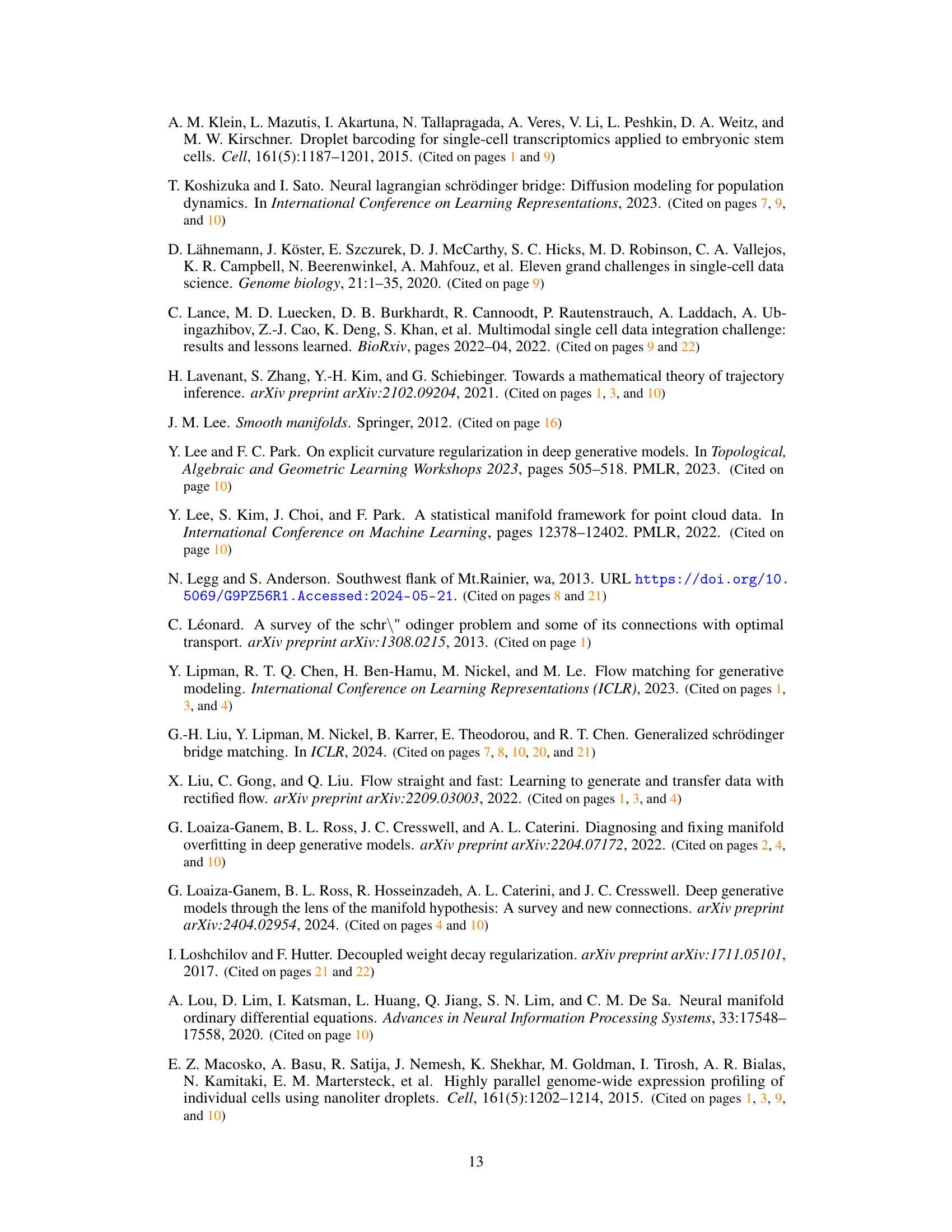
🔼 This table presents the Wasserstein-1 distance, a measure of similarity between probability distributions, calculated for various trajectory inference methods on three different single-cell datasets (Cite, EB, and Multi). The data was processed using principal component analysis (PCA) to reduce its dimensionality to the top 5 principal components. The left-out marginal approach was used for evaluation, where each model is trained on all but one time point and then tested on the excluded time point. The results are averaged over five independent runs, providing an estimate of the methods’ performance and stability. The lower the Wasserstein-1 distance, the better the method’s performance in reconstructing the trajectory.
read the caption
Table 4: Wasserstein-1 distance averaged over left-out marginals for 5-dim PCA representation of single-cell data for corresponding datasets. Results are averaged over 5 independent runs.
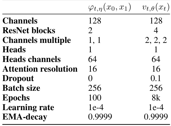
🔼 This table presents the hyperparameter settings used for the U-Net architecture in the unpaired image translation experiments on the AFHQ dataset. It shows the configurations for both the interpolant network (φτ,η (x0, x1)) and the vector field network (vt,θ (xt)). The hyperparameters include the number of channels, ResNet blocks, channel multiples, heads, attention resolution, dropout rate, batch size, epochs, and learning rate. These values were employed to train both the networks in the MFM model.
read the caption
Table 5: U-Net architecture hyperparameters for unpaired image translation on AFHQ.
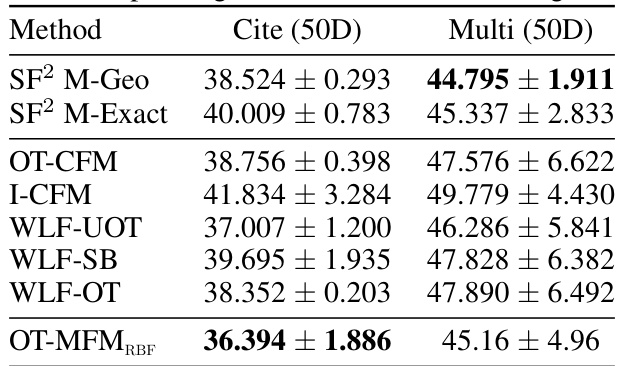
🔼 This table presents the Wasserstein-1 distance results for trajectory inference on single-cell data using 5 principal components. It compares the performance of OT-MFM against several baseline methods across three different single-cell datasets (Cite, EB, Multi). The lower the Wasserstein-1 distance, the better the performance in reconstructing the cell dynamics.
read the caption
Table 4: Wasserstein-1 distance averaged over left-out marginals for 5-dim PCA representation of single-cell data for corresponding datasets. Results are averaged over 5 independent runs.

🔼 This table shows the mean distance of the reconstructed trajectories from the sphere at time t=1/2. The results are averaged over five independent runs. It compares the performance of OT-CFM (Conditional Flow Matching with Euclidean metric) and OT-MFMLAND (Metric Flow Matching with LAND metric). Lower values indicate that the reconstructed trajectories are closer to the sphere, reflecting better performance.
read the caption
Table 7: Mean Distance of reconstructed trajectories at time 1/2 from the sphere. Results averaged over 5 runs.
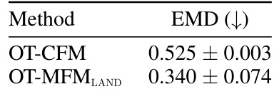
🔼 This table shows the Wasserstein-1 distance (EMD) between the reconstructed marginal distribution at time t=1/2 and the ground truth distribution for two different methods: OT-CFM (Euclidean baseline) and OT-MFMLAND (proposed method using LAND metric). The results are averaged over five independent runs, showing the performance of the proposed method in accurately reconstructing the target distribution compared to the Euclidean baseline.
read the caption
Table 8: Wasserstein-1 distance between reconstructed marginal at time 1/2 and ground-truth. Results averaged over 5 runs.
Full paper#
