TL;DR#
Long-term time series forecasting (LTSF) is challenging due to the complex, often chaotic nature of real-world data. Existing deep learning models struggle to capture the underlying dynamics of these series. This paper introduces Attraos, a novel model that addresses these issues.
Attraos incorporates chaos theory, treating real-world time series as low-dimensional observations from high-dimensional chaotic systems. The model uses phase space reconstruction and a multi-resolution dynamic memory unit to capture historical dynamical structures and attractor dynamics. A frequency-enhanced evolution strategy further enhances prediction accuracy. Attraos significantly outperforms existing methods on various datasets and requires far fewer parameters, demonstrating the effectiveness of chaos-based modeling for LTSF.
Key Takeaways#
Why does it matter?#
This paper is crucial for researchers in time series forecasting as it introduces a novel approach that leverages chaos theory for long-term prediction. Its efficient model, Attraos, outperforms existing methods and provides a new perspective using attractor dynamics. This opens up exciting avenues for research into chaos-based time series modeling, addressing the limitations of traditional methods, and offering potentially superior accuracy for complex, real-world datasets. The open-sourced code further enhances its impact by facilitating reproducibility and fostering collaboration within the research community.
Visual Insights#

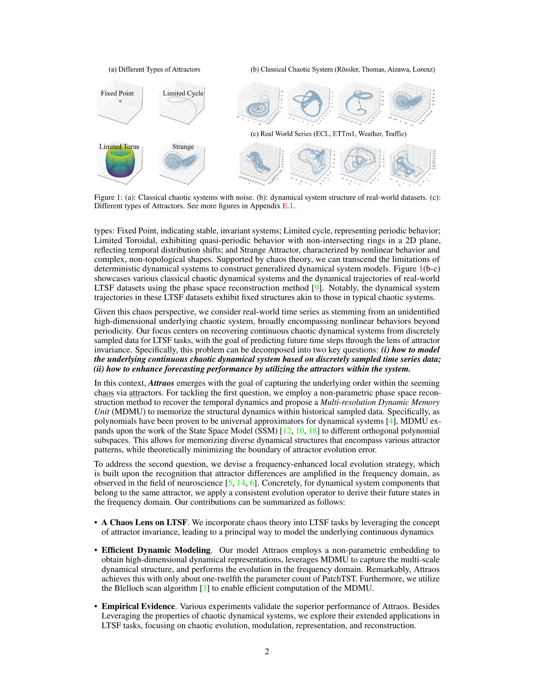
🔼 This figure shows different types of attractors in dynamical systems. (a) shows examples of attractors in classical chaotic systems with added noise, such as fixed points, limited cycles, limited tori, and strange attractors. (b) visualizes the structures of real-world time series datasets (ECL, ETTm1, Weather, Traffic) by using phase space reconstruction, which reveals that these time series exhibit similar structural patterns to those found in classical chaotic systems. (c) provides a summary of the different types of attractors and their characteristics.
read the caption
Figure 1: (a): Classical chaotic systems with noise. (b): dynamical system structure of real-world datasets. (c): Different types of Attractors. See more figures in Appendix E.1.

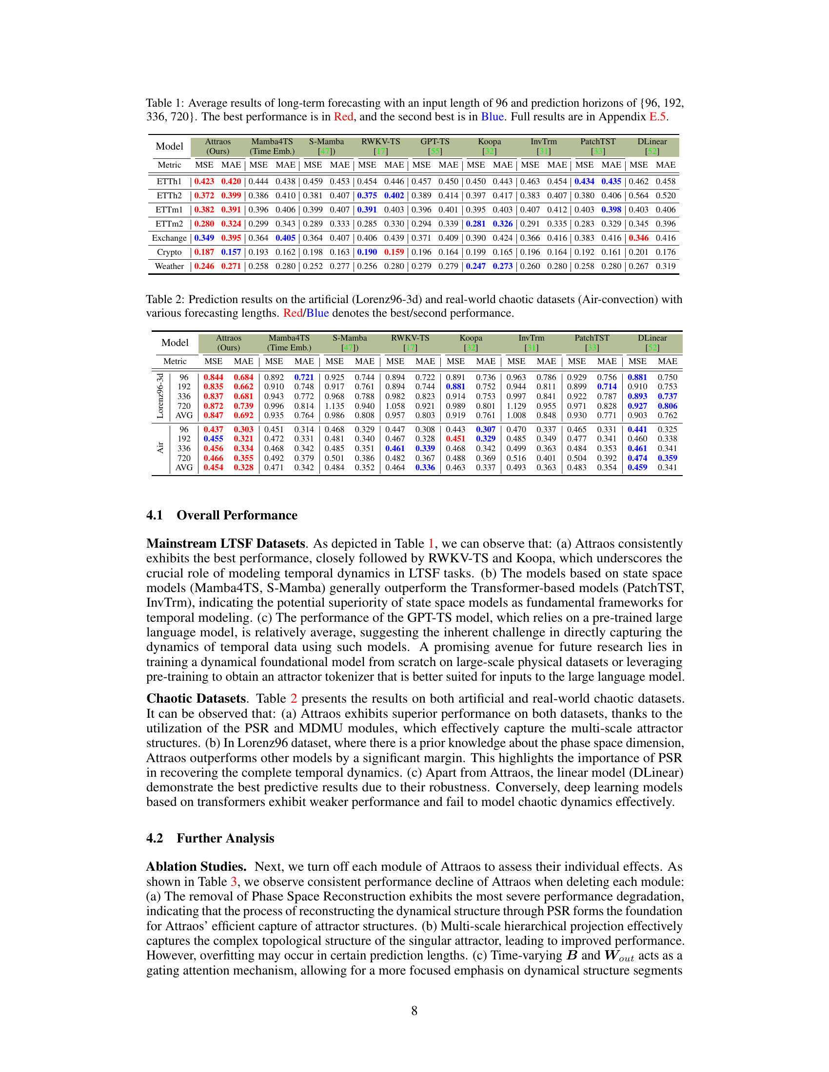
🔼 This table presents the average Mean Squared Error (MSE) and Mean Absolute Error (MAE) for various long-term time series forecasting models across multiple datasets. The input sequence length is fixed at 96 time steps, while the prediction horizon varies (96, 192, 336, and 720 steps). The best performing model for each dataset and prediction horizon is highlighted in red, and the second-best is highlighted in blue. For a complete breakdown of the results, including additional metrics, refer to Appendix E.5 of the paper.
read the caption
Table 1: Average results of long-term forecasting with an input length of 96 and prediction horizons of {96, 192, 336, 720}. The best performance is in Red, and the second best is in Blue. Full results are in Appendix E.5.
In-depth insights#
Chaos in LTSF#
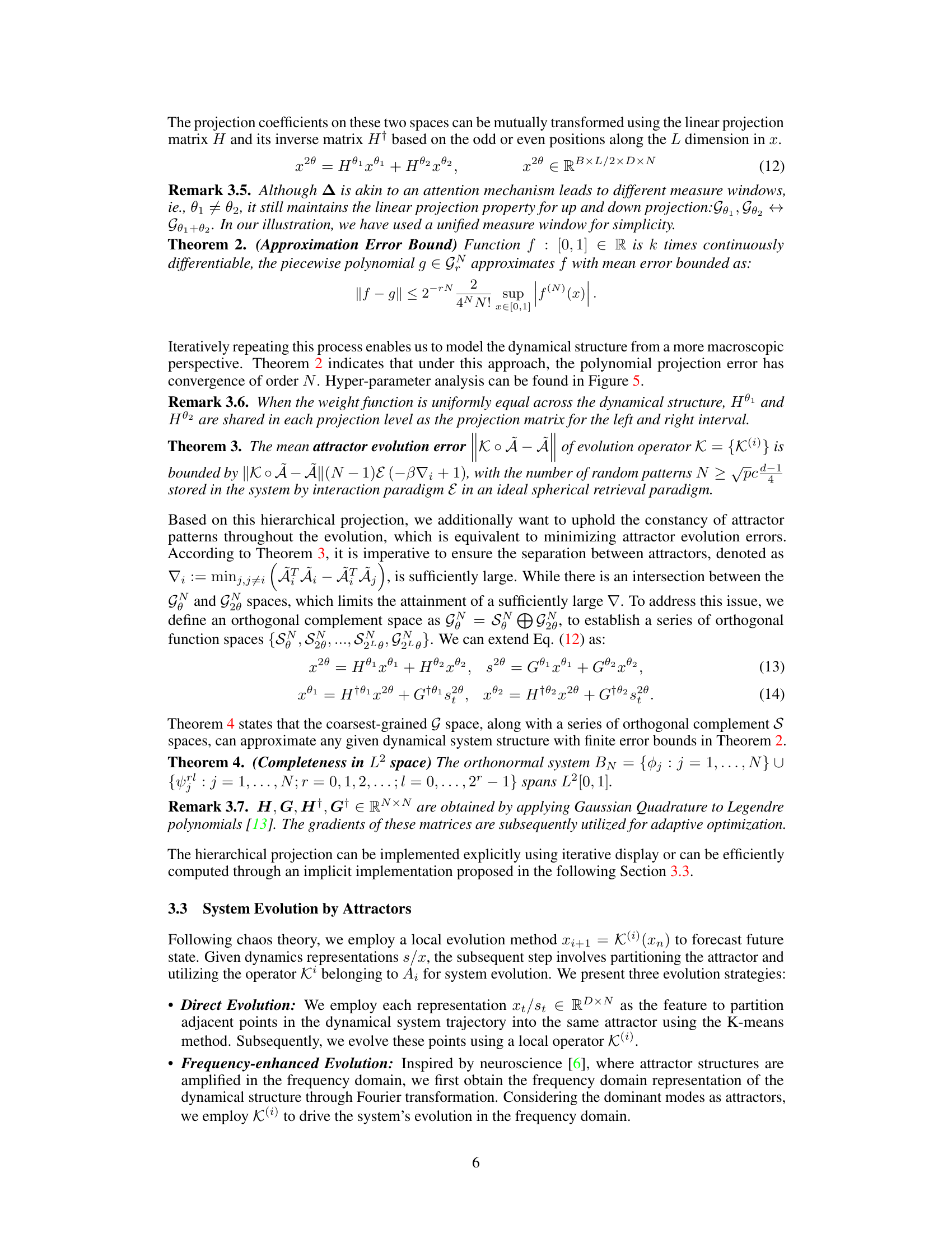
The application of chaos theory to long-term time series forecasting (LTSF) offers a novel perspective. Real-world time series, often exhibiting complex, seemingly unpredictable behavior, can be viewed as projections of underlying high-dimensional chaotic systems. This chaotic perspective suggests that traditional time-series methods, which typically assume linearity or simple non-linearity, may be inadequate. Instead, approaches focusing on the inherent dynamical systems, such as identifying attractors and their evolution, could be significantly more effective. Attractor invariance, a core principle in chaos theory, posits that the structure of an attractor, despite variations in observations, remains relatively stable. This stability enables the development of models that memorize and evolve the underlying dynamics, leading to improved long-term predictions. The application of chaos theory therefore introduces new modeling strategies and theoretical insights that hold the potential to revolutionize LTSF and to achieve more accurate and robust forecasting, especially for datasets with chaotic characteristics.
Attractor Memory#
The concept of ‘Attractor Memory’ in the context of long-term time series forecasting (LTSF) offers a novel approach to modeling complex temporal dynamics. Instead of treating time series as purely sequential data, this framework views them as manifestations of underlying continuous dynamical systems. The core idea revolves around the concept of attractors: stable patterns that emerge in the system’s trajectories after sufficient evolution. The method uses a multi-resolution dynamic memory unit (MDMU) to effectively store and recall these historical attractor structures, allowing the model to effectively learn long-term dependencies. This approach is especially powerful for handling chaotic systems because it focuses on learning stable attractor properties rather than being overly sensitive to short-term fluctuations. The frequency-enhanced local evolution strategy further refines the model’s predictions by leveraging attractor invariance. In essence, Attractor Memory provides a robust and efficient mechanism for LTSF tasks, particularly in scenarios involving noisy or chaotic datasets, by shifting focus from the detailed trajectory to the underlying, stable attractor patterns.
MDMU & FELE#
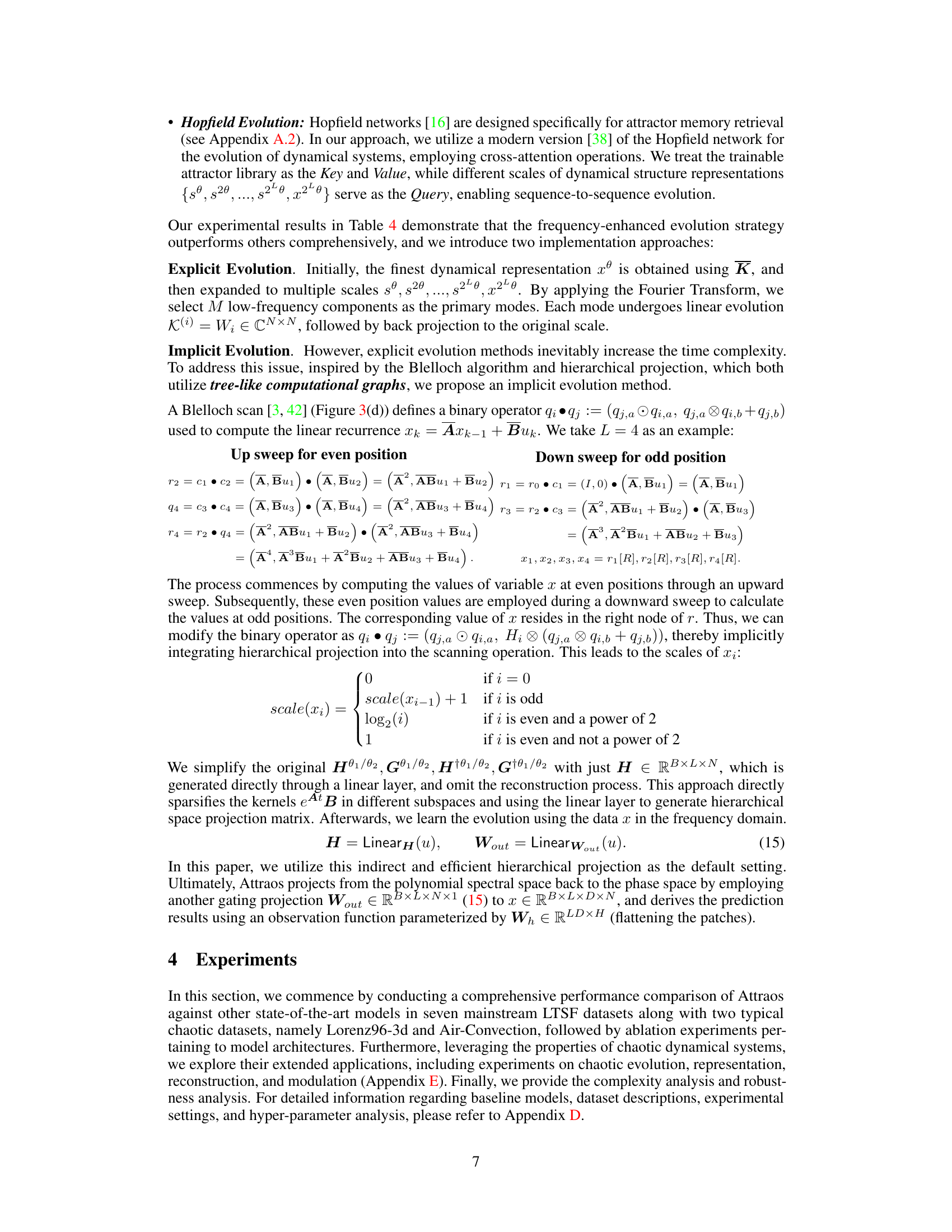
The proposed model innovatively combines a Multi-resolution Dynamic Memory Unit (MDMU) with a Frequency-Enhanced Local Evolution (FELE) strategy. MDMU addresses the challenge of capturing diverse dynamical structures within time series data by employing a multi-resolution approach, expanding upon state-space models (SSM). This allows it to effectively memorize historical dynamics across multiple scales, accommodating varied attractor patterns. FELE leverages the principle that attractor differences are amplified in the frequency domain, enhancing the model’s ability to differentiate and predict future states based on these nuanced differences. By operating in the frequency domain, FELE improves the efficiency and robustness of evolution. In essence, MDMU provides a comprehensive memory system, while FELE acts as a refined evolution engine, jointly contributing to more accurate and stable long-term time series forecasting. The combination of these two components offers a novel approach to modelling the complex, chaotic nature inherent in real-world data, overcoming limitations of traditional methods that struggle with capturing multi-scale dynamics and noisy observations.
Ablation Studies#
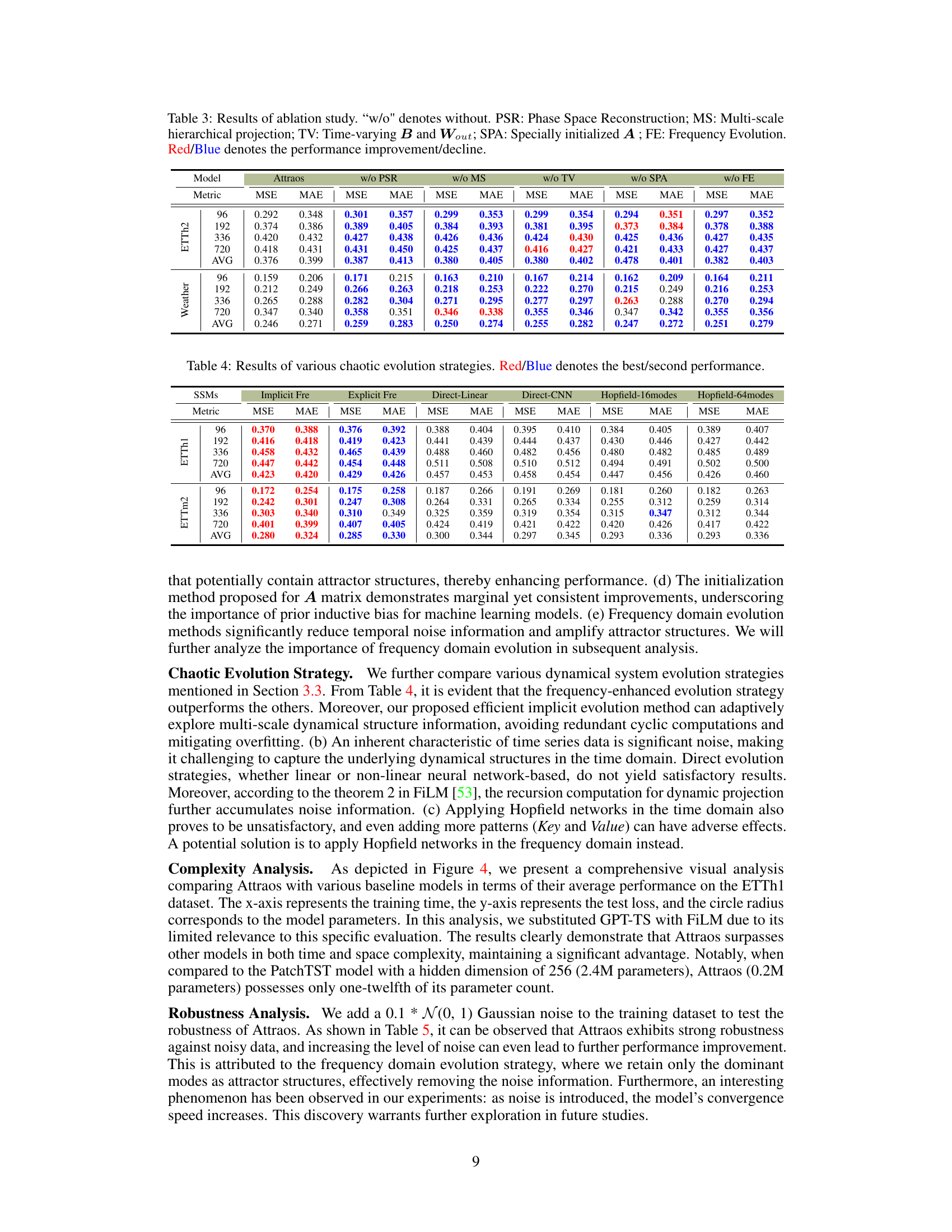
Ablation studies systematically remove or modify components of a model to assess their individual contributions. In this context, removing the Phase Space Reconstruction (PSR) module resulted in the most significant performance drop, highlighting its crucial role in capturing the underlying dynamical structures. The multi-scale hierarchical projection module, while effective, showed potential overfitting, suggesting further refinements. The time-varying parameters (B and Wout) acted as a gating attention mechanism, focusing on dynamic structure segments, and removing them reduced performance. Finally, the impact of the initialization method for matrix A was minor but consistent, indicating the value of careful parameter selection. Overall, the ablation study demonstrably proves the importance of each component in Attraos, providing valuable insights into its design and performance.
Future of LTSF#
The future of Long-Term Time Series Forecasting (LTSF) lies in addressing its current limitations and harnessing the power of emerging technologies. Improved handling of non-stationarity and noise is crucial, possibly through advanced methods like reservoir computing or hybrid models that combine statistical techniques with deep learning. Incorporating domain expertise and physical principles will allow for more accurate and explainable models, particularly in areas like climate prediction and financial markets. Hybrid models leveraging symbolic reasoning with neural networks could unlock better understanding of complex temporal patterns. The development of efficient and scalable algorithms is vital for dealing with the ever-increasing volume and complexity of time series data. Furthermore, research into causality within LTSF could lead to more robust and predictive models. Finally, exploring the potential of novel architectures like graph neural networks and transformers specialized for temporal data will continue to shape the field. Ultimately, the next generation of LTSF will likely be characterized by a combination of increased sophistication and explainability, enabling more reliable long-term predictions.
More visual insights#
More on figures

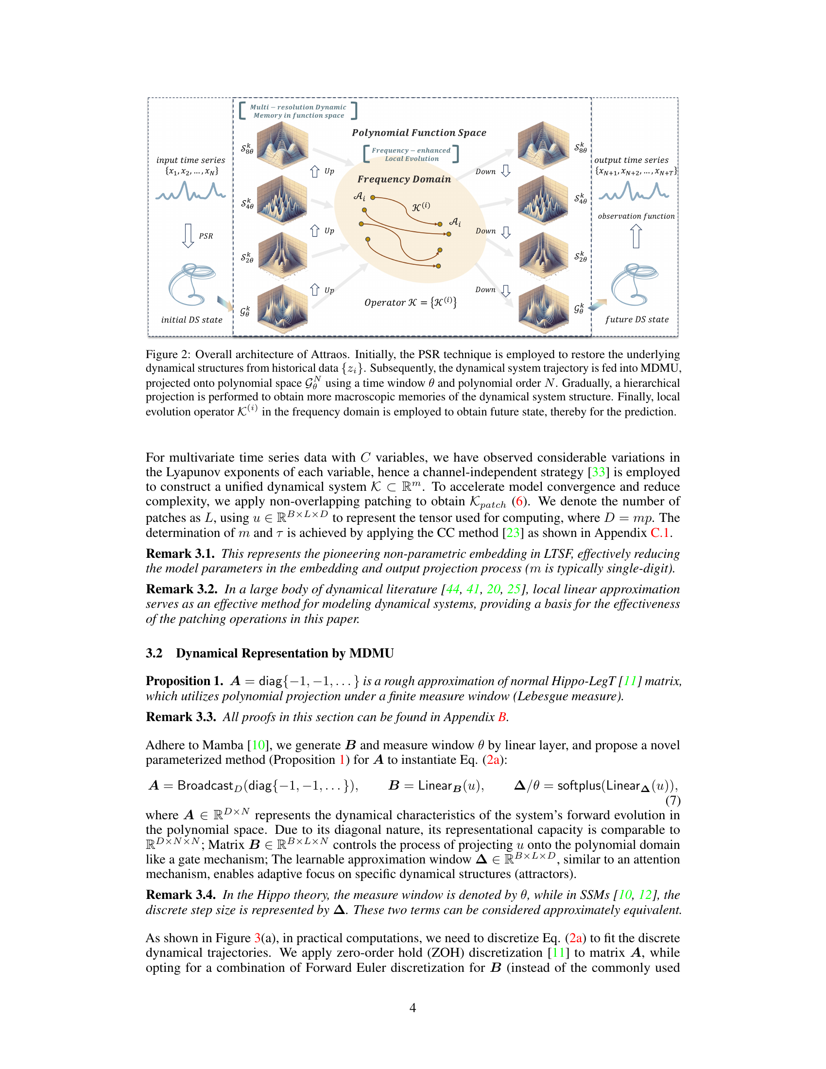
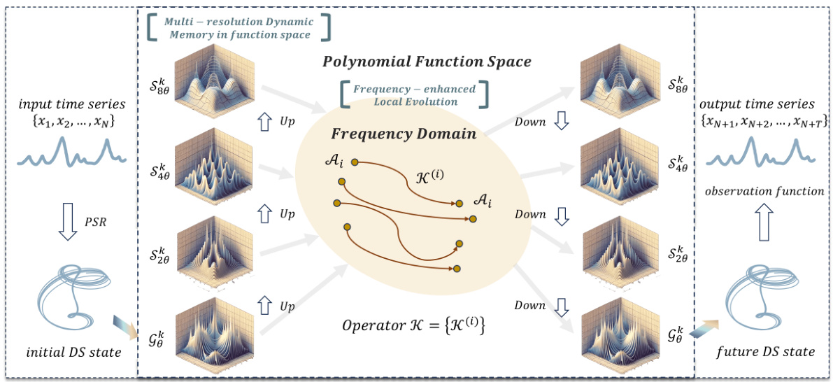
🔼 This figure illustrates the overall architecture of the Attraos model for long-term time series forecasting. It shows how the model uses Phase Space Reconstruction (PSR) to recover the underlying dynamical structures from historical data, employs a Multi-resolution Dynamic Memory Unit (MDMU) to memorize these structures, and uses a frequency-enhanced local evolution strategy to predict future states.
read the caption
Figure 2: Overall architecture of Attraos. Initially, the PSR technique is employed to restore the underlying dynamical structures from historical data {zi}. Subsequently, the dynamical system trajectory is fed into MDMU, projected onto polynomial space Gỗ using a time window θ and polynomial order N. Gradually, a hierarchical projection is performed to obtain more macroscopic memories of the dynamical system structure. Finally, local evolution operator K(i) in the frequency domain is employed to obtain future state, thereby for the prediction.
🔼 This figure illustrates the overall architecture of the Attraos model for long-term time series forecasting. The model consists of three main stages: 1) Phase Space Reconstruction (PSR) to reconstruct the underlying dynamical system from the input time series, 2) a Multi-resolution Dynamic Memory Unit (MDMU) to memorize the multi-scale dynamical structures using a hierarchical projection into polynomial function spaces, and 3) a frequency-enhanced local evolution strategy that operates in the frequency domain to predict future states.
read the caption
Figure 2: Overall architecture of Attraos. Initially, the PSR technique is employed to restore the underlying dynamical structures from historical data {zi}. Subsequently, the dynamical system trajectory is fed into MDMU, projected onto polynomial space Gỗ using a time window @ and polynomial order N. Gradually, a hierarchical projection is performed to obtain more macroscopic memories of the dynamical system structure. Finally, local evolution operator K(i) in the frequency domain is employed to obtain future state, thereby for the prediction.

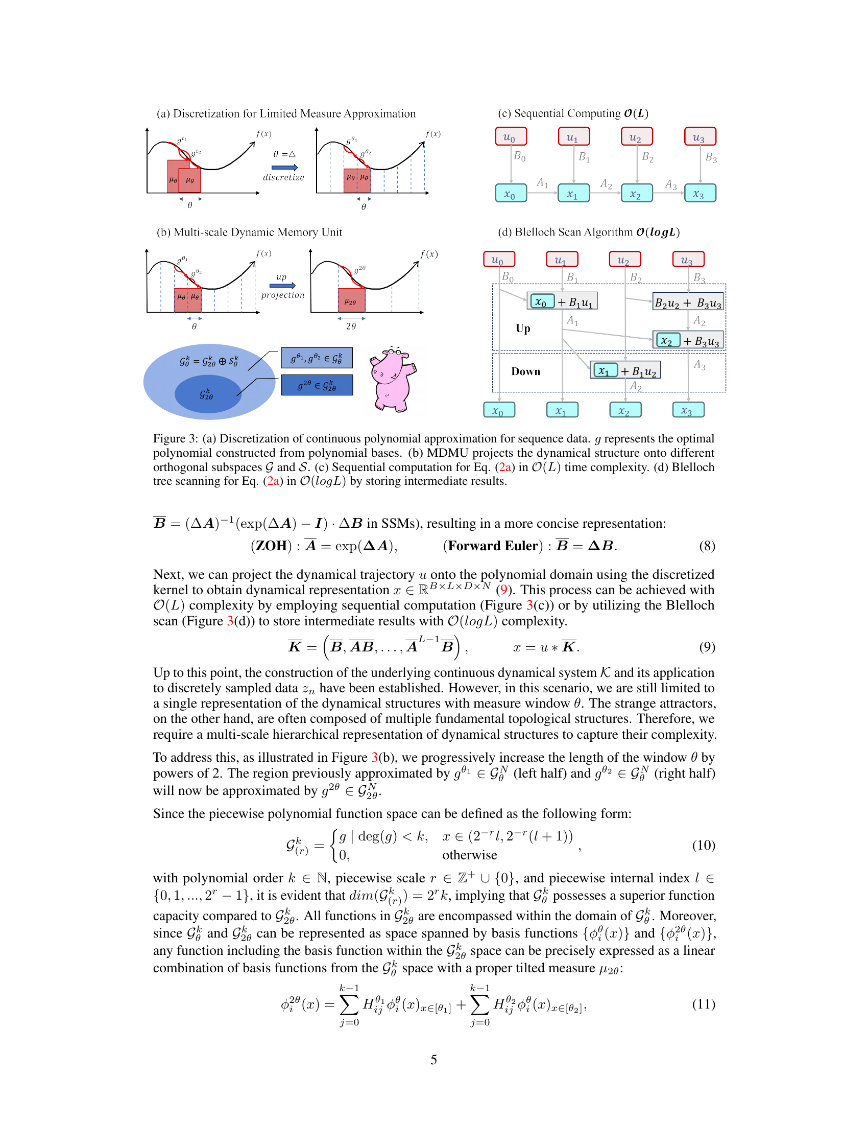
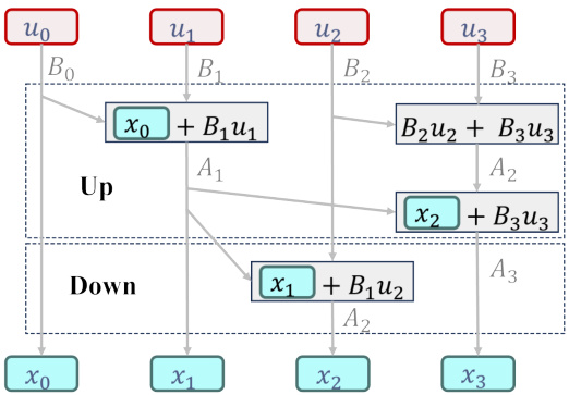
🔼 This figure shows the discretization of continuous polynomial approximation, the multi-scale dynamic memory unit (MDMU) that projects dynamical structures onto orthogonal subspaces, and the efficient computation methods used in the Attraos model, including sequential computation and Blelloch’s scan algorithm.
read the caption
Figure 3: (a) Discretization of continuous polynomial approximation for sequence data. g represents the optimal polynomial constructed from polynomial bases. (b) MDMU projects the dynamical structure onto different orthogonal subspaces G and S. (c) Sequential computation for Eq. (2a) in O(L) time complexity. (d) Blelloch Scan Algorithm O(logL) by storing intermediate results.

🔼 This figure shows the overall architecture of the Attraos model, which is composed of several key components: Phase Space Reconstruction (PSR), Multi-resolution Dynamic Memory Unit (MDMU), and Frequency-enhanced Local Evolution. PSR first transforms the input time series data into a higher-dimensional representation to capture the underlying dynamical structure. This representation is then fed into MDMU, which uses a multi-resolution approach to memorize diverse dynamical patterns. Finally, the model uses a frequency-enhanced local evolution strategy to predict future states based on learned dynamical structures in the frequency domain.
read the caption
Figure 2: Overall architecture of Attraos. Initially, the PSR technique is employed to restore the underlying dynamical structures from historical data {zi}. Subsequently, the dynamical system trajectory is fed into MDMU, projected onto polynomial space Gỗ using a time window @ and polynomial order N. Gradually, a hierarchical projection is performed to obtain more macroscopic memories of the dynamical system structure. Finally, local evolution operator K(i) in the frequency domain is employed to obtain future state, thereby for the prediction.
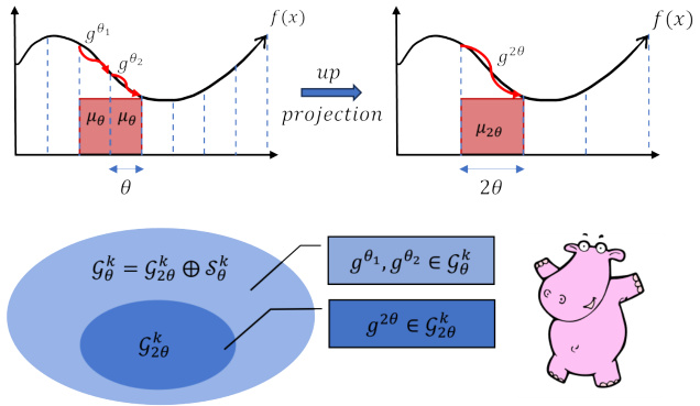
🔼 This figure illustrates the discretization of continuous polynomial approximation, the multi-scale dynamic memory unit (MDMU) and efficient computation methods for the dynamical representation in Attraos. Panel (a) shows the discretization process. Panel (b) depicts how MDMU projects dynamical structures onto different orthogonal subspaces. Panels (c) and (d) compare sequential computation and Blelloch scan algorithm for efficient computation.
read the caption
Figure 3: (a) Discretization of continuous polynomial approximation for sequence data. g represents the optimal polynomial constructed from polynomial bases. (b) MDMU projects the dynamical structure onto different orthogonal subspaces G and S. (c) Sequential computation for Eq. (2a) in O(L) time complexity. (d) Blelloch tree scanning for Eq. (2a) in O(logL) by storing intermediate results.
🔼 This figure illustrates the overall architecture of the Attraos model for long-term time series forecasting. It shows how the model processes input time series data through several key steps: Phase Space Reconstruction (PSR), Multi-resolution Dynamic Memory Unit (MDMU), and Frequency-enhanced Local Evolution. The PSR step reconstructs the underlying dynamical structures from the input time series. Then, MDMU projects this onto a polynomial space using a time window and polynomial order for hierarchical projection in order to obtain more macroscopic memories of the dynamical system structure. Finally, the frequency-enhanced local evolution operator predicts future states in the frequency domain, resulting in the output time series prediction.
read the caption
Figure 2: Overall architecture of Attraos. Initially, the PSR technique is employed to restore the underlying dynamical structures from historical data {zi}. Subsequently, the dynamical system trajectory is fed into MDMU, projected onto polynomial space Gỗ using a time window @ and polynomial order N. Gradually, a hierarchical projection is performed to obtain more macroscopic memories of the dynamical system structure. Finally, local evolution operator K(2) in the frequency domain is employed to obtain future state, thereby for the prediction.
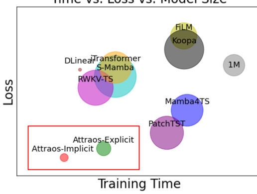
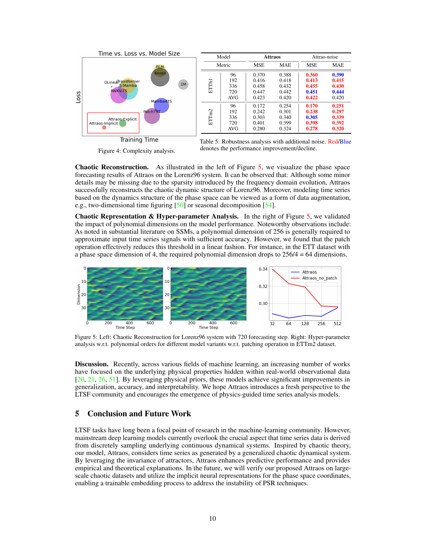
🔼 This figure compares the training time and test loss of various long-term time series forecasting models, including Attraos (both explicit and implicit versions), against several baselines. The size of each circle represents the number of model parameters. Attraos demonstrates superior performance with significantly fewer parameters compared to other models, particularly PatchTST.
read the caption
Figure 4: Complexity analysis.

🔼 This figure illustrates the overall architecture of Attraos, showing how it discretizes continuous polynomial approximation, uses the Multi-resolution Dynamic Memory Unit (MDMU) for dynamical representation, performs sequential and Blelloch scan algorithms for computation, and projects the dynamical structure onto orthogonal subspaces.
read the caption
Figure 3: (a) Discretization of continuous polynomial approximation for sequence data. g represents the optimal polynomial constructed from polynomial bases. (b) MDMU projects the dynamical structure onto different orthogonal subspaces G and S. (c) Sequential computation for Eq. (2a) in O(L) time complexity. (d) Blelloch Scan Algorithm O(logL)
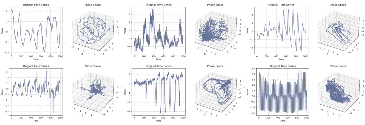
🔼 This figure visualizes the phase space structures of various real-world time series datasets. Each row represents a different dataset, showing both the original time series data (left) and its corresponding 3D phase space representation (right). The 3D phase space plots illustrate the trajectories of the data points, revealing the underlying dynamical structures and attractor patterns. Note that due to visualization limitations, the attractors for the time series might be of higher dimensions. Only slices of the attractors in the first three dimensions are shown.
read the caption
Figure 6: Dynamic structures of real-world data

🔼 This figure demonstrates the simulation process of generating time series data from a high-dimensional chaotic system (Lorenz96). (a) shows the trajectory of the Lorenz63 system in a 3D phase space. (b) illustrates how the 40D Lorenz96 system is mapped to a 3D space using a random initialized linear neural network, which represents the observation function h. The visualization in (b) shows a chaotic system trajectory in 3D. Finally, (c) presents a 1D visualization of the three dimensions obtained from the mapping process.
read the caption
Figure 7: Simulation for Lorenz96
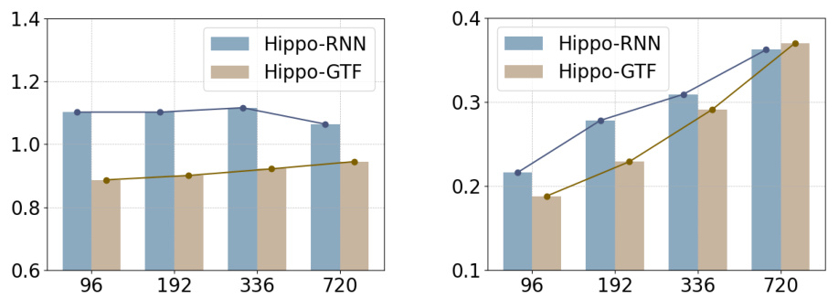
🔼 This figure shows the performance comparison of two methods (Hippo-RNN and Hippo-GTF) using MSE as the metric. The left subplot displays the results for the Lorenzo96 dataset, while the right subplot shows the results for the Weather dataset. The x-axis represents the forecasting window length, and the y-axis represents the MSE values. The results demonstrate the impact of teaching forcing on the predictive performance of the methods.
read the caption
Figure 8: Performance comparison about teaching forcing, measured by MSE. Left: Lorenzo96 dataset. Right: Weather dataset.
More on tables

🔼 This table presents the average Mean Squared Error (MSE) and Mean Absolute Error (MAE) for various long-term time series forecasting models across multiple datasets. The input sequence length is 96 time steps and the prediction horizons are 96, 192, 336, and 720 steps. The best and second-best performing models for each dataset and prediction horizon are highlighted in red and blue respectively. More detailed results are provided in Appendix E.5.
read the caption
Table 1: Average results of long-term forecasting with an input length of 96 and prediction horizons of {96, 192, 336, 720}. The best performance is in Red, and the second best is in Blue. Full results are in Appendix E.5.

🔼 This table presents the average Mean Squared Error (MSE) and Mean Absolute Error (MAE) for various long-term time series forecasting models on eight benchmark datasets. The input sequence length was 96 time steps, and the prediction horizons were 96, 192, 336, and 720 steps. The best and second-best results for each dataset and prediction horizon are highlighted in red and blue respectively. Complete results can be found in Appendix E.5.
read the caption
Table 1: Average results of long-term forecasting with an input length of 96 and prediction horizons of {96, 192, 336, 720}. The best performance is in Red, and the second best is in Blue. Full results are in Appendix E.5.

🔼 This table presents the results of an ablation study conducted on the Attraos model. It shows the impact of removing each module of the model (PSR, MS, TV, SPA, and FE) individually on the model’s performance, measured by Mean Squared Error (MSE) and Mean Absolute Error (MAE). The results are shown for different prediction horizons (96, 192, 336, and 720) and aggregated as average for two datasets, ETTh1 and Weather. Red color indicates performance improvement, while blue indicates performance decline compared to the full model.
read the caption
Table 3: Results of ablation study. 'w/o' denotes without. PSR: Phase Space Reconstruction; MS: Multi-scale hierarchical projection; TV: Time-varying B and Wout; SPA: Specially initialized A; FE: Frequency Evolution. Red/Blue denotes the performance improvement/decline.

🔼 This table presents the average Mean Squared Error (MSE) and Mean Absolute Error (MAE) of different long-term time series forecasting models on eight benchmark datasets, with input length of 96 and prediction horizons ranging from 96 to 720. The best and second-best performing models for each dataset and horizon are highlighted in red and blue, respectively. Further details are provided in Appendix E.5.
read the caption
Table 1: Average results of long-term forecasting with an input length of 96 and prediction horizons of {96, 192, 336, 720}. The best performance is in Red, and the second best is in Blue. Full results are in Appendix E.5.

🔼 This table presents the average Mean Squared Error (MSE) and Mean Absolute Error (MAE) for various long-term time series forecasting models on eight benchmark datasets (ETTh1, ETTh2, ETTm1, ETTm2, Exchange, Crypto, Weather, and ECL). The input length for all models was 96 time steps, and the prediction horizons were 96, 192, 336, and 720. The best performing model for each dataset and horizon is highlighted in red, while the second-best is in blue. The full results, including additional metrics, are provided in Appendix E.5.
read the caption
Table 1: Average results of long-term forecasting with an input length of 96 and prediction horizons of {96, 192, 336, 720}. The best performance is in Red, and the second best is in Blue. Full results are in Appendix E.5.

🔼 This table presents the average Mean Squared Error (MSE) and Mean Absolute Error (MAE) for various long-term time series forecasting models on eight different datasets. The input sequence length was 96 time steps, and predictions were made for horizons of 96, 192, 336, and 720 steps. The best-performing model for each dataset and prediction horizon is highlighted in red, and the second-best is in blue. Detailed results, including all metrics for all prediction horizons can be found in Appendix E.5. The table compares Attraos to several existing state-of-the-art methods.
read the caption
Table 1: Average results of long-term forecasting with an input length of 96 and prediction horizons of {96, 192, 336, 720}. The best performance is in Red, and the second best is in Blue. Full results are in Appendix E.5.
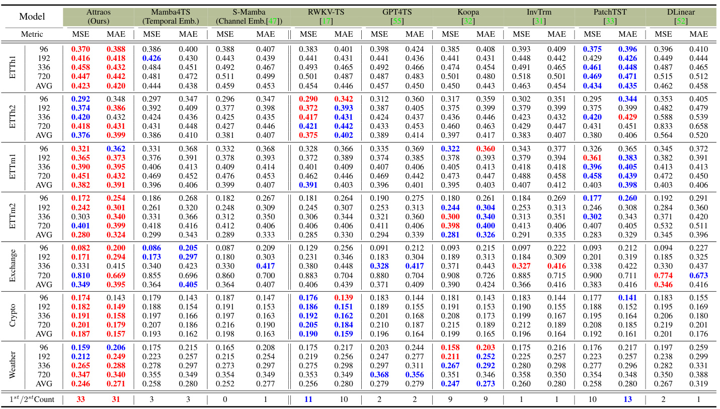
🔼 This table presents the results of a multivariate long-term time series forecasting experiment using various models on mainstream datasets. The input sequence length was 96, and prediction horizons were 96, 192, 336, and 720. The best-performing model is highlighted in boldface, with the second-best underlined. The lower portion of the table shows results from a variant using kernel functions for multivariate handling.
read the caption
Table 7: Multivariate long-term series forecasting results in mainstream datasets with input length is 96 and prediction horizons are {96, 192, 336, 720}. The best model is in boldface, and the second best is underlined. The bottom part introduces the variable Kernel for multivariate variables.
Full paper#

