Active Sequential Posterior Estimation for Sample-Efficient Simulation-Based Inference

↗ OpenReview ↗ NeurIPS Homepage ↗ Chat

TL;DR

#

Key Takeaways

#

Why does it matter?

#

This paper is crucial for researchers in simulation-based inference and related fields because it presents ASNPE, a novel sample-efficient method. It offers significant improvements in high-dimensional problems where computational resources are limited and addresses a critical challenge in making inference under complex models more feasible. This opens up avenues for applications across scientific domains requiring complex simulation models, such as traffic network optimization and more.

Visual Insights

#

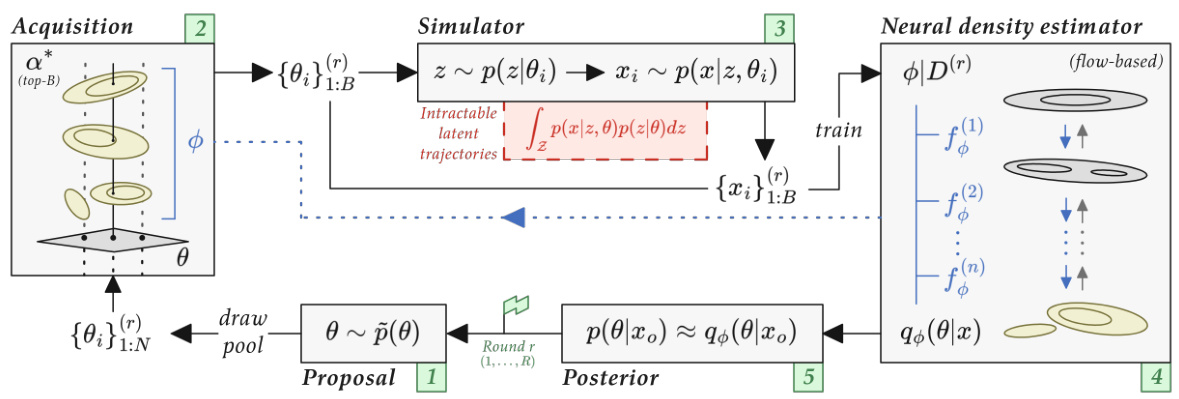
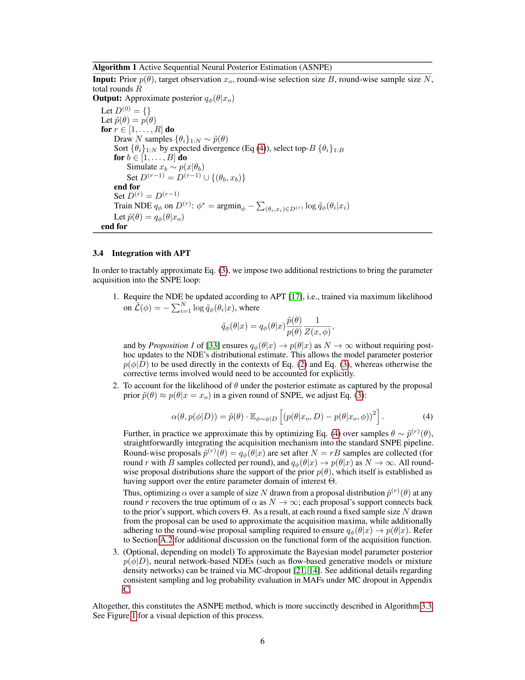
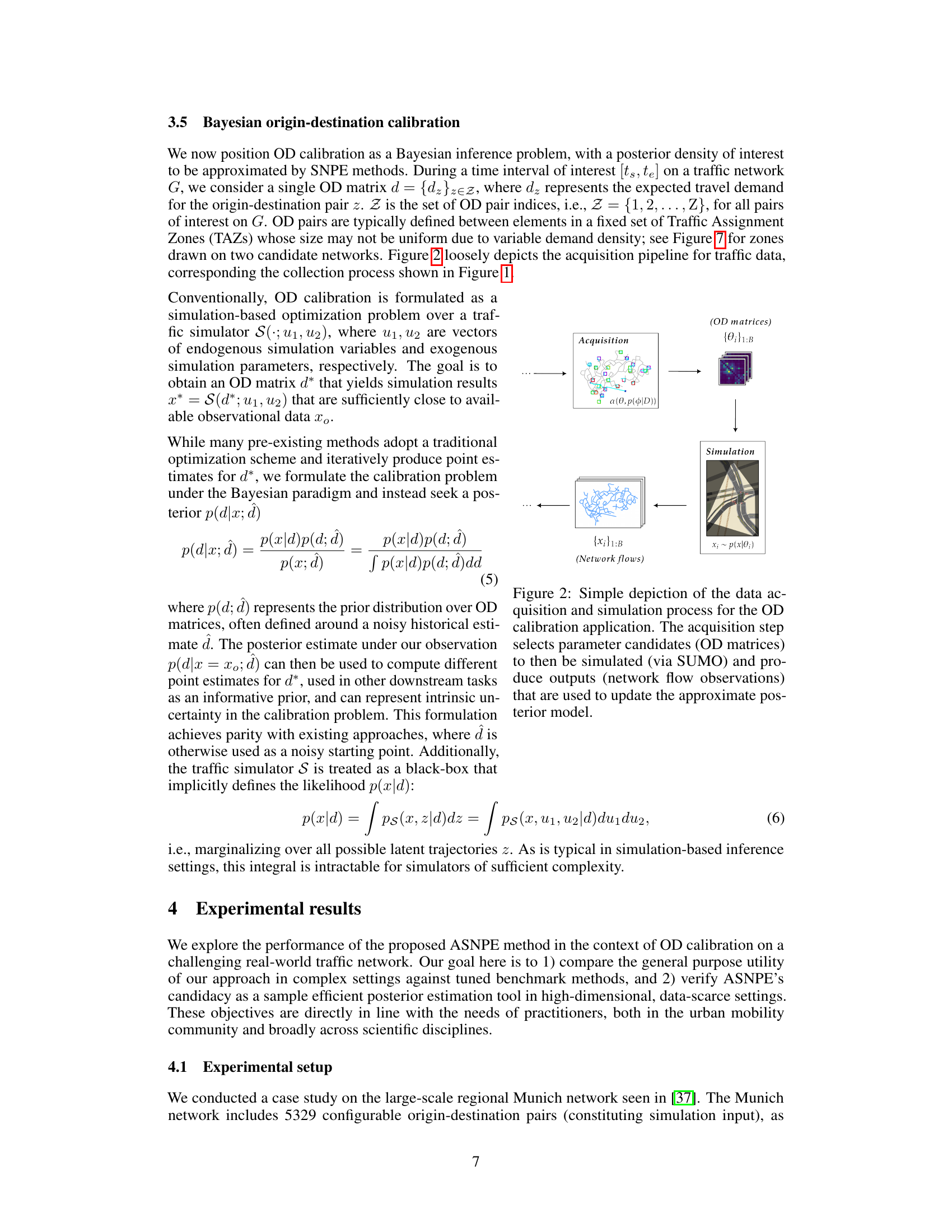
This figure shows a high-level overview of the Active Sequential Neural Posterior Estimation (ASNPE) method. It illustrates how samples are drawn from a proposal distribution, filtered based on an acquisition function, and then used to train a neural density estimator to approximate the posterior distribution. The updated posterior is then used to generate a new proposal distribution for the next iteration.

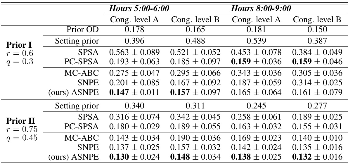
This table presents the Root Mean Squared Normalized Error (RMSNE) scores achieved by different methods on the Munich traffic network for OD calibration. It compares SPSA, PC-SPSA, MC-ABC, SNPE, and ASNPE across different congestion levels and time intervals, using two different prior distributions. The results show the RMSNE values and their standard deviations over five trial runs, highlighting the performance of each method in terms of accuracy and convergence.

In-depth insights

#

Active SNI

#

Active Sequential Neural Posterior Estimation (ASNPE) presents a novel approach to Simulation-Based Inference (SBI). ASNPE enhances sample efficiency by integrating active learning, strategically selecting simulation parameters to maximize information gain. Unlike passive methods that blindly sample, ASNPE intelligently targets areas of high uncertainty in the posterior distribution, focusing computational resources on the most informative simulations. This targeted approach leads to improved accuracy of the posterior estimate with fewer simulations, making it especially suitable for high-dimensional problems or computationally expensive simulators. The active learning strategy seamlessly integrates into existing SBI pipelines, enhancing their performance rather than requiring a complete overhaul. ASNPE’s effectiveness is demonstrated in a real-world application—origin-destination calibration in a large-scale traffic network—as well as on standard SBI benchmarks, showcasing its broad applicability and superior performance compared to traditional and state-of-the-art SBI methods. The key innovation is its ability to directly quantify uncertainty in the neural density estimator (NDE) and use this quantification to guide the active selection process.

ASNPE Method

#

The ASNPE method, an enhancement of SNPE, introduces active learning to improve sample efficiency in simulation-based inference. Instead of passively sampling parameters, ASNPE actively selects parameters expected to maximize information gain by targeting epistemic uncertainty in the neural density estimator (NDE). This is achieved by defining an acquisition function that quantifies the expected reduction in uncertainty across different NDE parameterizations, focusing on areas where the NDE is less certain. The method leverages Bayesian flow-based generative models for NDEs, facilitating efficient uncertainty quantification and integration with the active learning scheme. Integration with APT (Automatic Posterior Transformation) ensures convergence to the true posterior. The acquisition function efficiently incorporates both the uncertainty and likelihood of a parameter sample, providing a principled approach to guide simulation runs. Efficiency and scalability are key advantages, particularly when dealing with computationally expensive simulators and high-dimensional problems. The effectiveness is demonstrated via OD calibration, a high-dimensional inverse problem; ASNPE outperforms existing methods, showing significant improvement in sample efficiency and accuracy.

OD Calibration

#

The paper explores OD (Origin-Destination) calibration, a crucial task in transportation planning. High-fidelity traffic simulators, while powerful, pose challenges due to their computational cost and the complexity of inverse problems. The authors frame OD calibration as a Bayesian inference problem, leveraging active learning to improve the efficiency of sample acquisition from the simulator. This active learning strategy aims to select the most informative simulation parameters, improving the accuracy and efficiency of posterior estimation. Neural density estimators are used to approximate the posterior distribution, allowing for uncertainty quantification. The proposed method, ASNPE, demonstrates its effectiveness, outperforming state-of-the-art benchmarks on a large-scale real-world traffic network. ASNPE’s sample efficiency is a significant advantage, particularly relevant given the computational expense of high-fidelity traffic simulators. The paper highlights the scalability and flexibility of the approach, showcasing the potential to make OD calibration more efficient and practical in real-world applications.

SBI Benchmarks

#

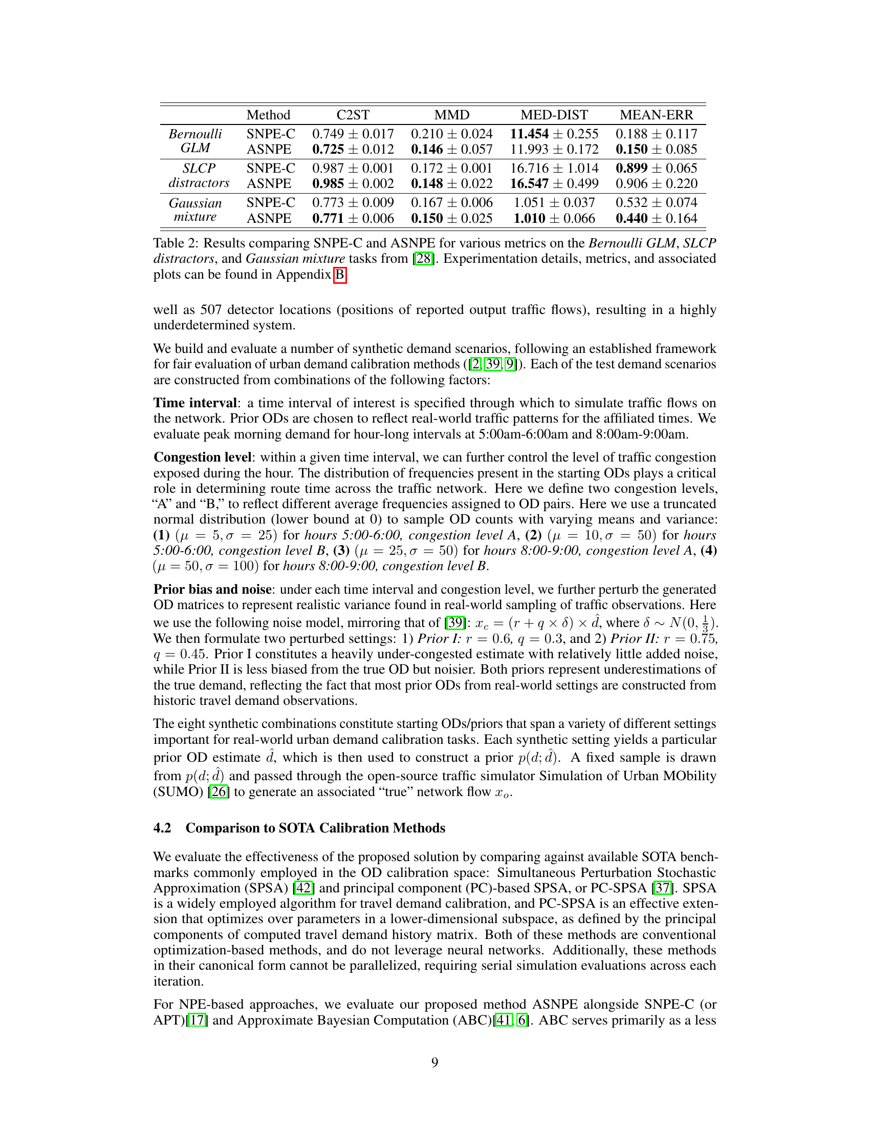
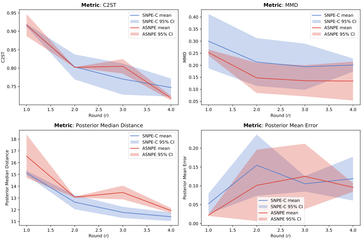
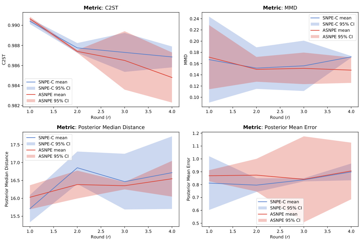
The section on SBI benchmarks is crucial for evaluating the generalizability and robustness of the proposed ASNPE method. It allows for a comparison against existing state-of-the-art (SOTA) methods on established, standardized tasks. The choice of benchmarks is vital; they should represent diverse problem structures and complexities to demonstrate ASNPE’s effectiveness beyond the specific application of OD matrix calibration. Results on these benchmarks provide strong evidence of ASNPE’s performance advantage over other methods, especially in terms of sample efficiency. However, a detailed analysis of the specific benchmark challenges and ASNPE’s performance across various metrics (like C2ST, MMD, mean error) is needed to fully understand its strengths and weaknesses. The inclusion of a quantitative comparison and a discussion of the factors contributing to ASNPE’s success or limitations in each benchmark scenario is critical for a comprehensive assessment. Finally, the selection and presentation of results should clearly highlight ASNPE’s performance gains and their statistical significance.

Future Work

#

Future research directions stemming from this work could explore several promising avenues. Extending ASNPE to handle even higher-dimensional problems is crucial, potentially through more sophisticated dimensionality reduction techniques or improved acquisition function approximations. Investigating alternative neural density estimators, beyond the flow-based models employed here, could also enhance performance and scalability. A deeper analysis of the acquisition function’s sensitivity to hyperparameters and its robustness under varied simulation scenarios would be valuable. Developing theoretical guarantees for ASNPE’s sample efficiency remains an important open question. Finally, applying ASNPE to a wider range of scientific domains, beyond traffic modeling, would demonstrate its generalizability and impact. The success of ASNPE hinges on the balance between efficient exploration and exploitation; future studies should systematically explore this tradeoff.

More visual insights

#

More on figures

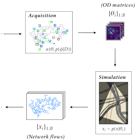
This figure shows a high-level overview of the Active Sequential Neural Posterior Estimation (ASNPE) pipeline. It illustrates how samples are actively selected based on an acquisition function, simulated using a model, and then used to train a neural density estimator to approximate the posterior distribution. The updated posterior is then used to guide the selection of subsequent samples, creating a sequential process.

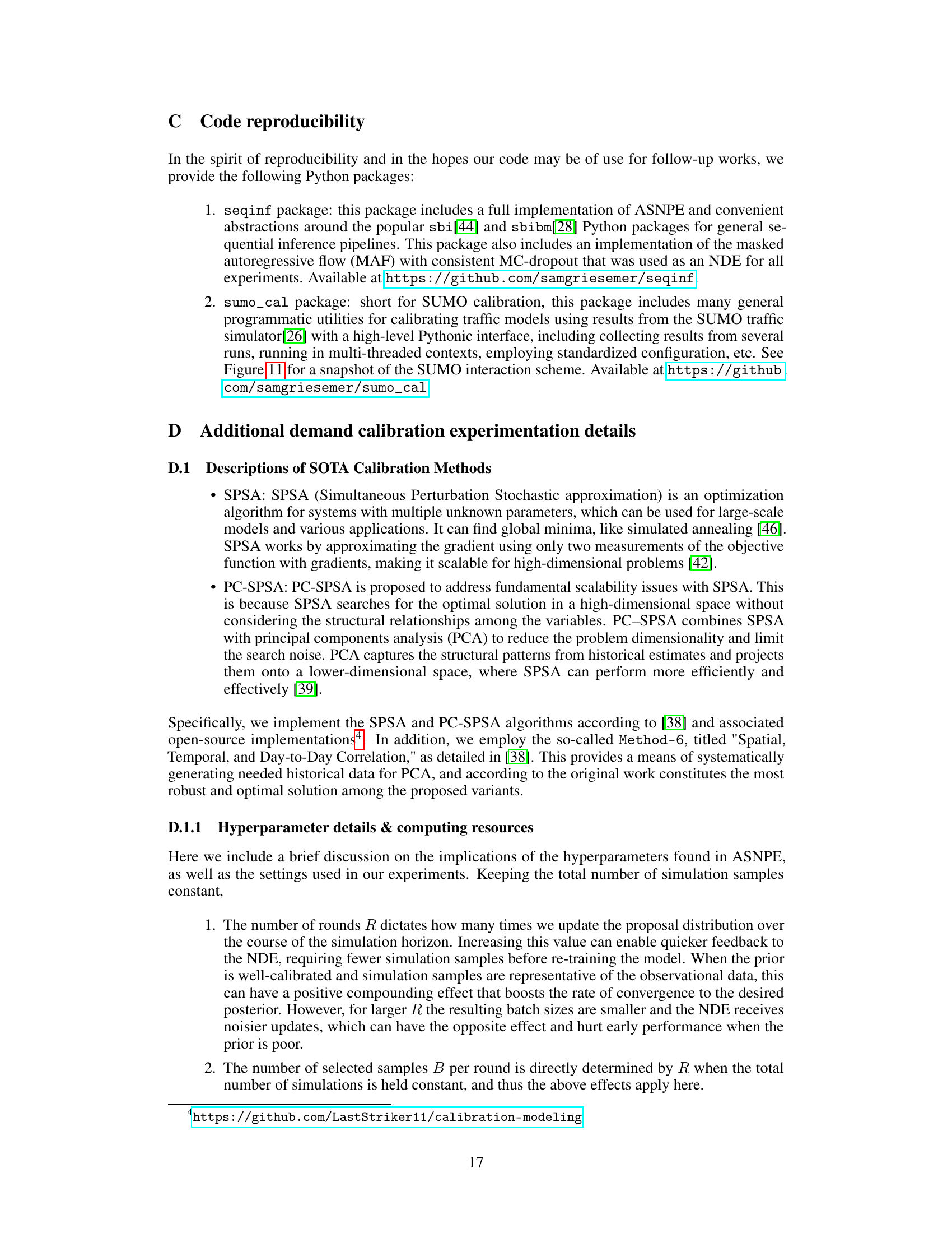
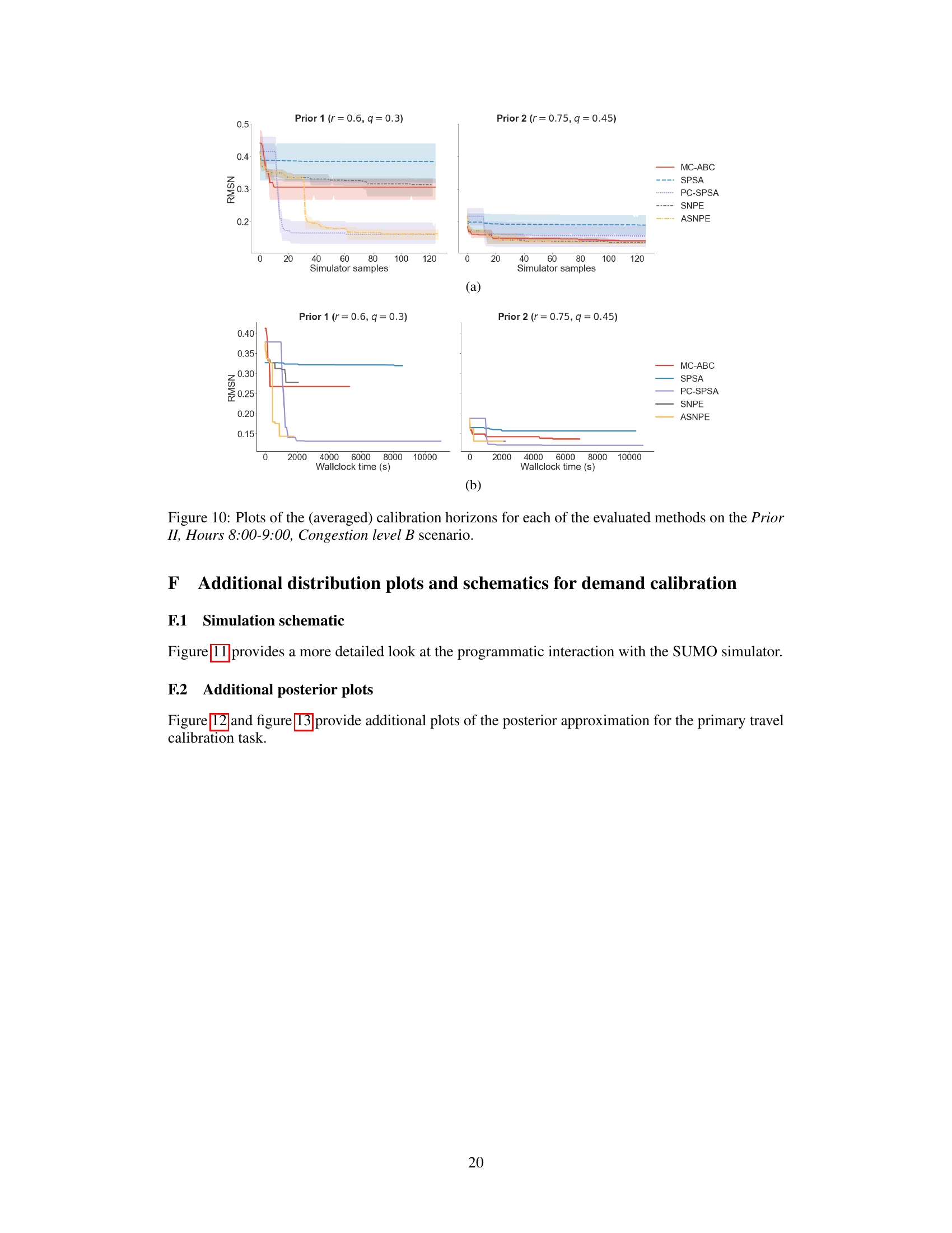
This figure compares different methods for calibrating origin-destination matrices in a traffic simulation model. It shows the root mean squared normalized error (RMSNE) achieved by each method over a simulation horizon of 128 samples. Subplot (a) shows the RMSNE as a function of the number of simulation samples, while subplot (b) shows the RMSNE as a function of wall-clock time. The figure demonstrates that the proposed ASNPE method achieves lower RMSNE scores than other methods, both in terms of the number of samples and wall-clock time, especially when using NPE-based methods that allow for parallelization.

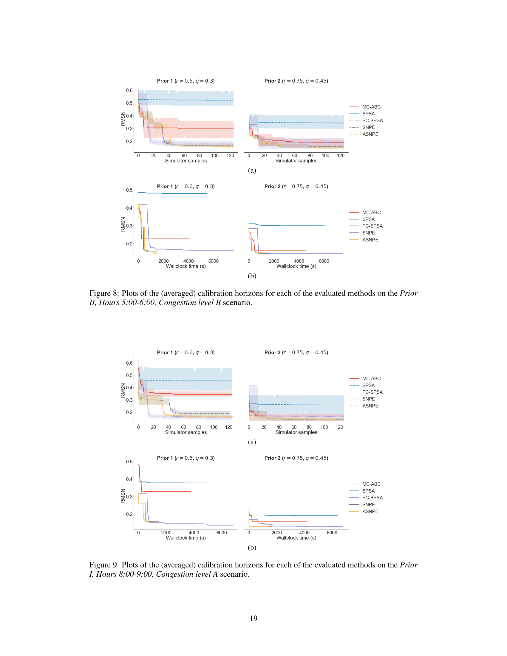
This figure compares the performance of different OD calibration methods across two metrics: RMSNE score and wall-clock time. It shows that ASNPE achieves lower RMSNE scores and faster convergence compared to other methods, highlighting its efficiency in a parallel computing environment. The plots are broken down by different prior settings and congestion levels to showcase the method’s robustness and effectiveness under varying conditions.

This figure shows a high-level overview of the Active Sequential Neural Posterior Estimation (ASNPE) method. It illustrates how samples are drawn from sequentially updated proposal distributions, filtered based on an acquisition function, and passed through a simulator to generate data for training a neural density estimator. The trained estimator then conditions on the target observation to produce the next round’s proposal distribution. The process iteratively refines the posterior estimation.

This figure shows a high-level overview of the ASNPE (Active Sequential Neural Posterior Estimation) pipeline. It illustrates how samples are actively selected based on an acquisition function, then simulated to improve the accuracy of the posterior estimation. The process iteratively refines the proposal distribution to focus on more informative parameter regions.

This figure is a flowchart showing the steps involved in the proposed active sequential neural posterior estimation (ASNPE) method. It illustrates how the algorithm iteratively refines the posterior distribution by actively selecting informative samples, simulating them using the model, and updating the neural density estimator (NDE). The key steps are: 1) drawing samples from a proposal distribution, 2) filtering samples based on an acquisition function, 3) simulating the filtered samples, 4) training the NDE using the generated data, 5) updating the proposal distribution based on the NDE, and iterating steps 1-5. This active sampling approach is designed to improve sample efficiency, especially for high-dimensional problems.

This figure compares the performance of different OD calibration methods (SPSA, PC-SPSA, MC-ABC, SNPE, ASNPE) across 128 simulation samples. It shows the root mean squared normalized error (RMSNE) achieved over time, both in terms of the number of simulation samples and the wall-clock time taken. The plots illustrate the impact of parallel processing capabilities of NPE-based methods (SNPE and ASNPE) and the variability in simulation runtimes, providing insights into the trade-offs between sample efficiency and computational cost.

This figure compares the performance of different OD calibration methods (MC-ABC, SPSA, PC-SPSA, SNPE, and ASNPE) in terms of root mean squared normalized error (RMSNE) achieved within a simulation horizon of 128 samples. Subplot (a) shows the RMSNE scores as a function of the number of simulation samples, while subplot (b) shows the same scores as a function of wall-clock time. The variability in line lengths highlights the parallel processing capabilities of NPE-based methods and the noise in simulation times due to varying input parameters.

This figure compares the performance of different OD calibration methods (SPSA, PC-SPSA, MC-ABC, SNPE, ASNPE) in terms of RMSNE scores achieved within a 128-sample simulation budget for a specific scenario (Prior 1, Hours 5:00-6:00, Congestion level A). Subplot (a) shows RMSNE scores over the number of simulation samples, while subplot (b) shows the same scores against wall-clock time, highlighting the impact of parallelization and simulation runtime variability. Error bars represent bootstrapped 95% confidence intervals.

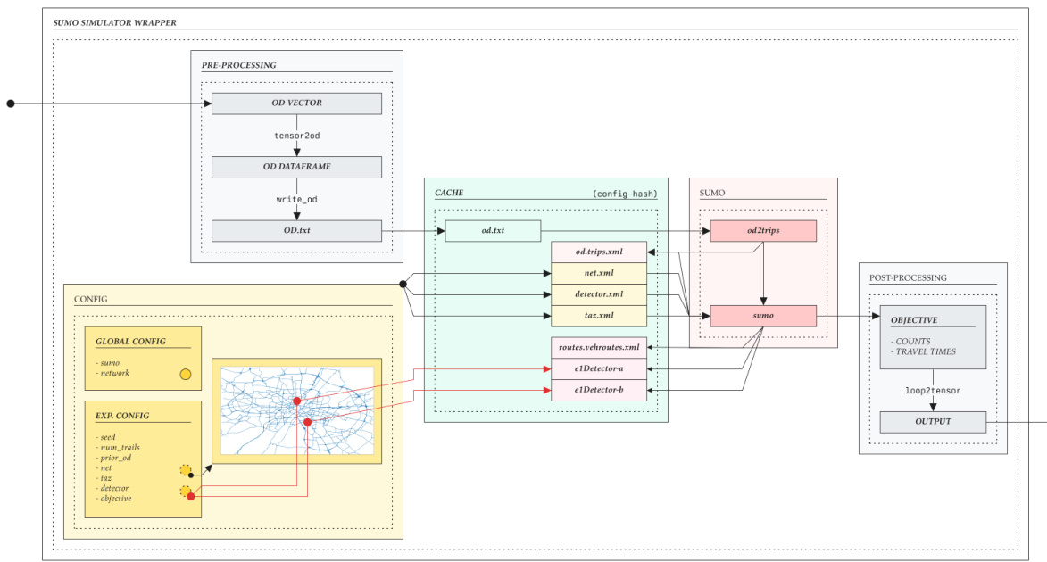
This figure shows a high-level overview of the Active Sequential Neural Posterior Estimation (ASNPE) pipeline. It illustrates how samples are drawn from sequentially updated proposal distributions, filtered using an acquisition function, and passed through a simulator to generate pairs for posterior estimation. The process iteratively refines the posterior approximation using active learning.

This figure shows pairwise density plots visualizing the 20-dimensional final approximate posterior generated by the ASNPE method. It specifically visualizes the results for the first scenario from the experimental setup (Prior I, Hours 5:00-6:00, Congestion level A). Each plot shows the relationship between two dimensions of the posterior distribution, providing insights into the correlations and the overall shape of the posterior.

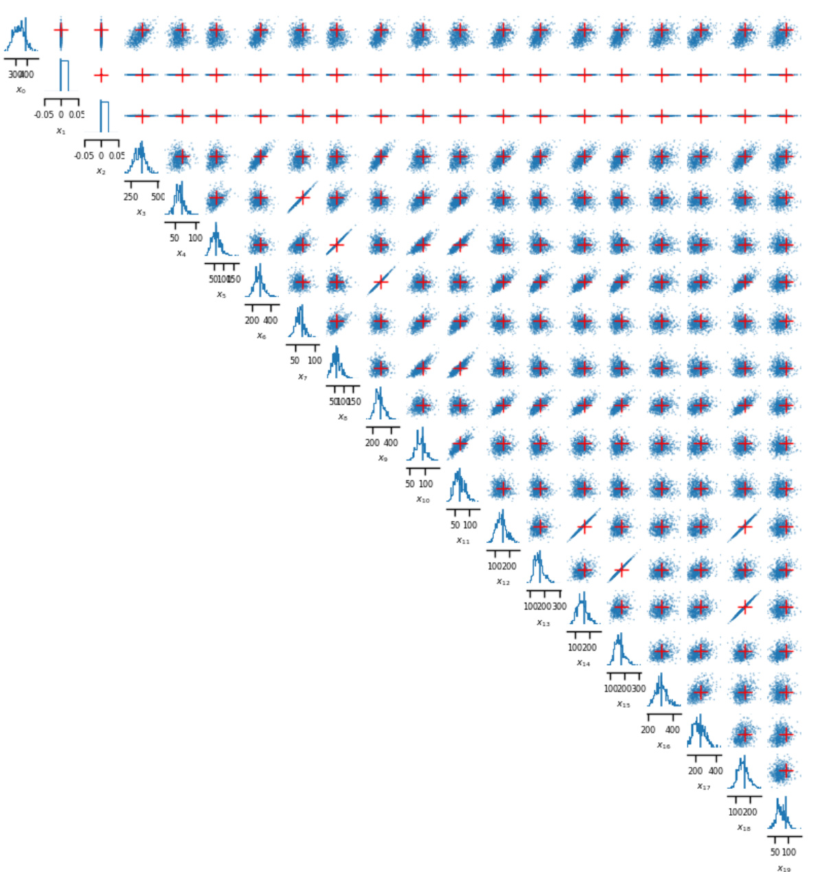
This figure shows pairwise density plots visualizing the relationships between 20 dimensions of the posterior distribution generated by the ASNPE method. Each plot shows the marginal distribution of a pair of dimensions, with the density represented by color intensity. The red crosses indicate the observed data point (x0), which serves as a reference point for evaluating how well the model captures the underlying distribution.

Full paper

#