↗ OpenReview ↗ NeurIPS Homepage ↗ Chat
TL;DR#
Hierarchical clustering, a fundamental task in unsupervised learning, traditionally faces challenges with discrete optimization methods being computationally expensive and continuous methods failing to guarantee alignment with discrete optima. Existing approaches also struggle to scale effectively to large datasets. This limits the accuracy and applicability of hierarchical clustering across various domains.
The paper introduces Expected Probabilistic Hierarchies (EPH), addressing these issues by learning hierarchies through probabilistic modeling and optimizing expected scores. EPH uses differentiable hierarchy sampling, allowing for end-to-end gradient descent optimization, and an unbiased subgraph sampling technique to handle large datasets efficiently. Experimental results demonstrate EPH’s superiority over existing methods on various benchmarks. The work provides a significant advancement in developing more effective and scalable hierarchical clustering algorithms.
Key Takeaways#
Why does it matter?#
This paper is crucial for researchers in unsupervised learning and hierarchical clustering because it introduces a novel and scalable probabilistic model (EPH) that overcomes limitations of existing methods. EPH’s end-to-end differentiability enables gradient-based optimization, and its unbiased sampling strategy allows for efficient scaling to large datasets. This opens new avenues for developing more accurate and efficient hierarchical clustering algorithms with applications in various fields.
Visual Insights#

This figure provides a visual overview of the Expected Probabilistic Hierarchies (EPH) model. The process begins with a probabilistic hierarchy, which is used to sample multiple discrete hierarchies. Concurrently, a subgraph is sampled from the input graph data. The sampled discrete hierarchies and subgraph are used to compute expected scores (e.g., Exp-Das, Exp-TSD). These scores are then averaged to compute the loss, which is used to update the parameters of the probabilistic hierarchy via backpropagation. This iterative process refines the probabilistic hierarchy until convergence.

This table compares four different cost functions used for hierarchical clustering: Soft-Das, Exp-Das, Soft-TSD, and Exp-TSD. It shows whether each function is a minimization or maximization problem, whether it’s convex or concave with respect to the parameters A and B that describe the probabilistic hierarchy, whether it always results in an integral solution, whether its optimum is equal to the optimal discrete solution, and whether the optimal value of the soft-score aligns with the optimal value of the corresponding discrete score. The table highlights the key theoretical properties of each cost function, indicating their suitability for optimization.
In-depth insights#
EPH: A Novel Method#
The heading “EPH: A Novel Method” suggests a research paper introducing a new technique called EPH. EPH likely represents an algorithm or framework designed to solve a specific problem within a field like machine learning, data mining, or graph analysis. The “novel” aspect implies that this method offers significant improvements over existing approaches, perhaps by addressing limitations or improving efficiency. The paper likely details the method’s theoretical foundation, including its mathematical formulation and algorithms. Experimental results are likely presented to demonstrate the efficacy of EPH, comparing its performance to other state-of-the-art techniques. The evaluation probably focuses on metrics relevant to the task EPH aims to solve, such as accuracy, efficiency, or scalability. A significant contribution of EPH would be its innovative approach to the problem and its potential for broader applications across diverse domains.
Expected Score Optim.#
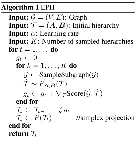
The heading ‘Expected Score Optim.’ suggests a methodology focusing on optimizing a probabilistic score, rather than directly optimizing a deterministic objective function. This is particularly relevant in the context of unsupervised learning problems, like hierarchical clustering, where the search space of discrete hierarchies is vast and complex. By working with expected scores, one can utilize techniques from continuous optimization, such as gradient descent, opening up efficient methods unavailable to traditional discrete optimization approaches. This probabilistic framework allows for learning hierarchies through differentiable hierarchy sampling, a technique that leverages continuous relaxations to facilitate gradient-based optimization. A key advantage is that the expected scores may directly translate to the optimal values of their discrete counterparts, providing a theoretical grounding for using continuous methods to approximate solutions to discrete problems. The approach likely involves sampling from a probability distribution over hierarchies, estimating the score for each sample, and then using this empirical estimate to guide the optimization process, making it computationally more tractable than exhaustively searching the discrete space.
Differentiable Sampling#
Differentiable sampling techniques are crucial for training models with discrete latent variables, a common challenge in areas like hierarchical clustering. The core idea is to approximate discrete sampling processes with continuous, differentiable counterparts, allowing for the application of gradient-based optimization methods. This is essential because standard backpropagation cannot directly handle discrete variables. The Gumbel-softmax trick and related methods are prominent examples, providing a way to sample from a categorical distribution while maintaining differentiability. However, directly applying these techniques to complex structures like hierarchical trees can be challenging. The success of differentiable sampling hinges on finding effective approximations that balance accuracy and computational efficiency. The trade-off between these two factors is crucial, impacting the model’s ability to learn meaningful representations. For complex structures, unbiased sampling methods are particularly important to guarantee that the resulting gradients accurately reflect the underlying discrete optimization problem. Therefore, methods like unbiased subgraph sampling become significant for handling large datasets where exhaustive enumeration of all possibilities would be computationally prohibitive. Careful consideration must be given to the selection of appropriate approximations, and the effects of biased gradients on the final model’s performance needs to be studied.
Scalable Subgraph#
The concept of “Scalable Subgraph” in the context of hierarchical clustering suggests a method to efficiently handle large datasets. The core idea likely revolves around breaking down the computational complexity of evaluating similarity scores or objective functions. Instead of processing the entire graph, a smaller, representative subgraph is sampled and used for computation. This approach trades off perfect accuracy for significant gains in speed, allowing the algorithm to scale to datasets that would otherwise be intractable. The scalability is achieved by strategically choosing the subgraph to capture the essential structure of the larger graph. Different sampling techniques, like random edge sampling or more sophisticated methods that consider node centrality or community structure, may be employed to ensure the representative nature of the subgraph. Unbiased sampling is crucial to avoid introducing systematic errors or biases that could impact the accuracy of the hierarchical clustering results. Furthermore, the choice of subgraph size needs careful consideration, balancing the trade-off between computational cost and the information loss due to the subsampling.
Future Research#
Future research directions stemming from this work on Expected Probabilistic Hierarchies (EPH) could explore several promising avenues. Improving the scalability of EPH for extremely large datasets remains a key challenge; investigating more sophisticated sampling techniques or approximation methods is crucial. Extending EPH to handle various data modalities beyond graphs and vectors, such as text or time-series data, would broaden its applicability. A deeper theoretical analysis of the model’s convergence properties and the impact of different sampling strategies would strengthen the EPH foundation. Finally, applying EPH to real-world problems and developing novel evaluation metrics specifically tailored for probabilistic hierarchies would further validate its effectiveness and impact.
More visual insights#
More on figures

This figure demonstrates a scenario where the Flexible Probabilistic Hierarchy (FPH) method fails to find the optimal hierarchy that minimizes the Dasgupta cost, unlike the Expected Probabilistic Hierarchies (EPH) method. It uses an unweighted K4 graph (complete graph with 4 nodes) as an example. FPH, using a continuous relaxation, achieves a Dasgupta cost of 4.0 after discretization, while the optimal discrete hierarchy has a cost of 3.0. However, EPH successfully identifies this optimal discrete hierarchy with a cost of 3.0, showcasing its advantage over FPH in finding the optimal discrete hierarchy.

This figure shows the impact of two hyperparameters on the performance of the Expected Probabilistic Hierarchies (EPH) model for hierarchical clustering. The left panel illustrates how the normalized Dasgupta cost changes with varying numbers of sampled hierarchies used during training. Different colors represent different datasets. The right panel examines the effect of the number of sampled edges on the normalized Dasgupta cost, comparing EPH against the average linkage algorithm (AL) and a full graph training (FG). The normalization ensures that each dataset’s mean is zero and standard deviation is one, allowing for comparison across different datasets.
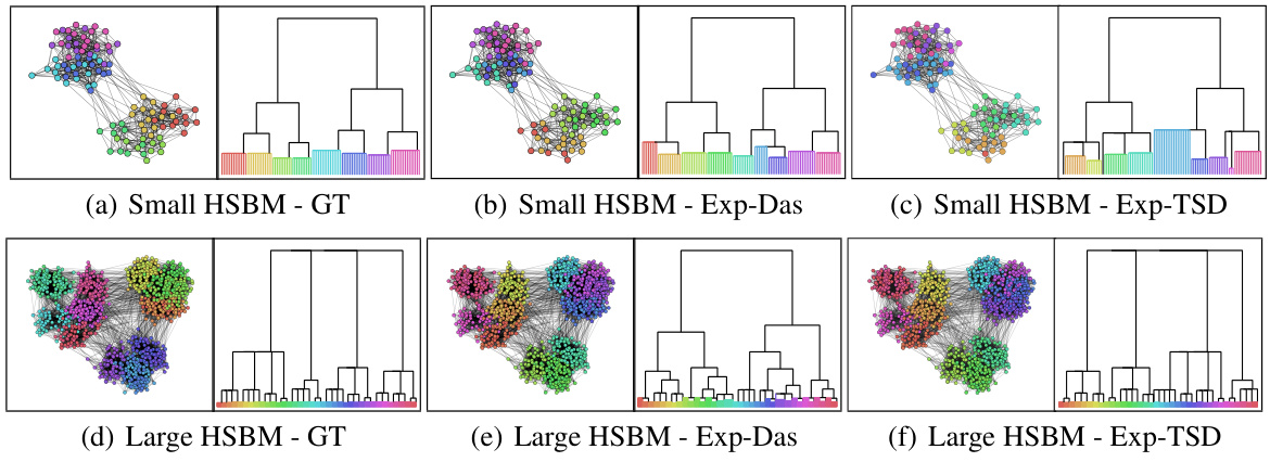
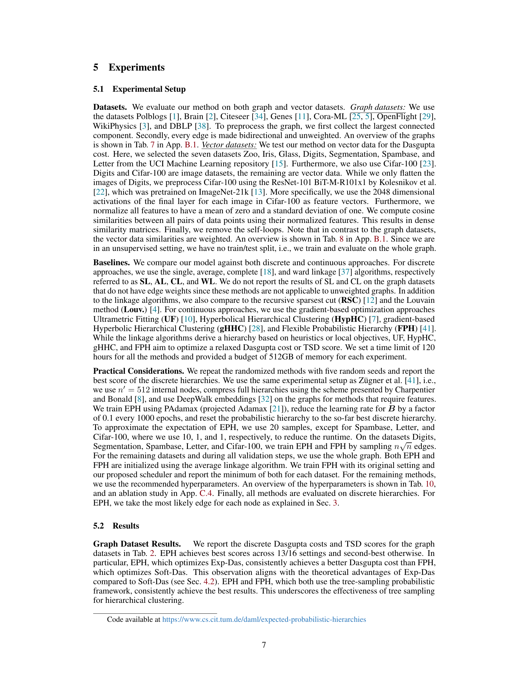
This figure visualizes the ground truth and the hierarchical clustering results obtained by EPH for both small and large Hierarchical Stochastic Block Models (HSBMs). The top row shows the results for a small HSBM, while the bottom row shows the results for a larger HSBM. Within each row, the leftmost panel displays the ground truth community structure (GT), the middle panel shows the dendrogram generated by EPH using the expected Dasgupta cost (Exp-Das), and the rightmost panel shows the dendrogram produced by EPH using the expected Tree-Sampling Divergence (Exp-TSD). The color-coding in the dendrograms represents the clusters identified by the algorithm. The figure provides a visual comparison of how well EPH’s clustering results align with the ground truth community structure for different network sizes and using different evaluation metrics.

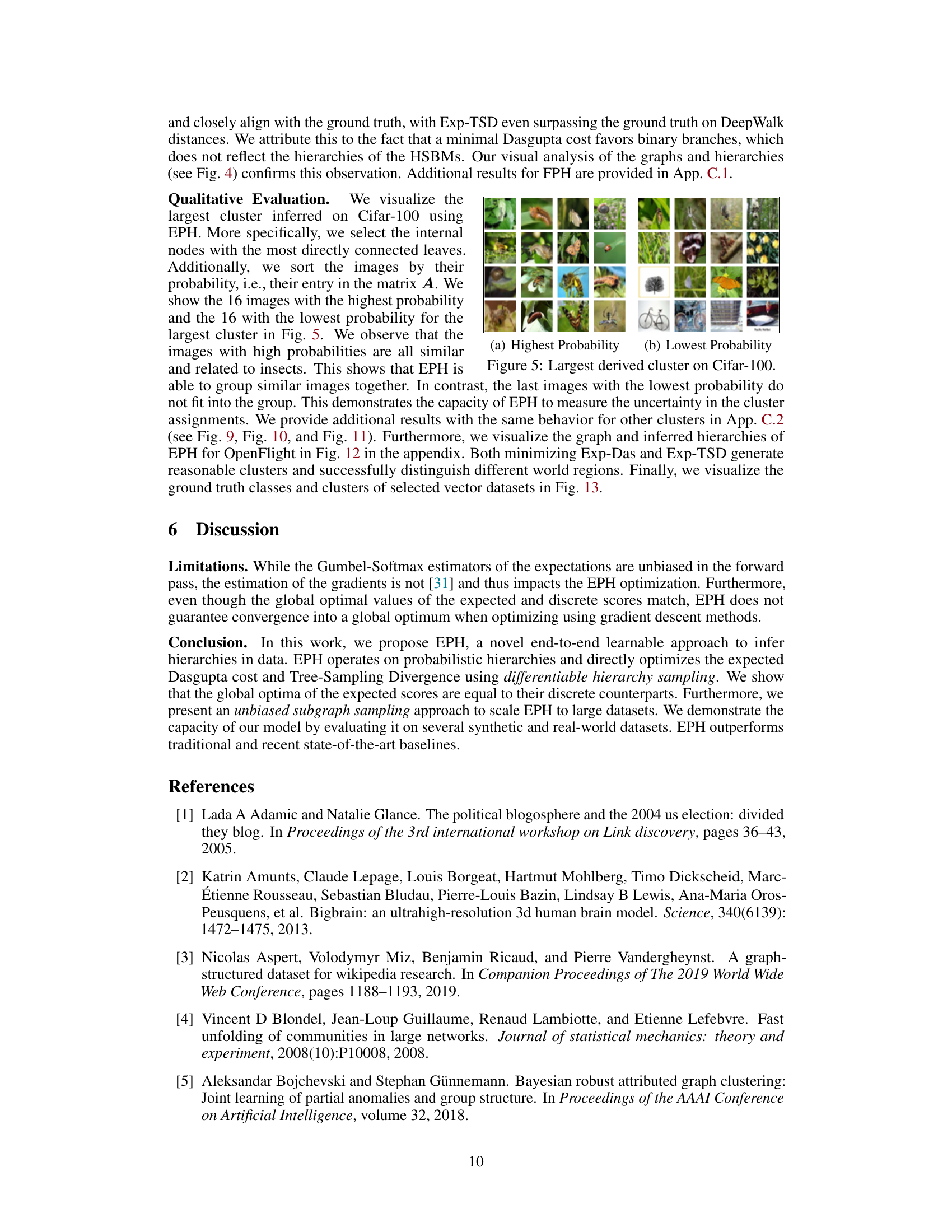
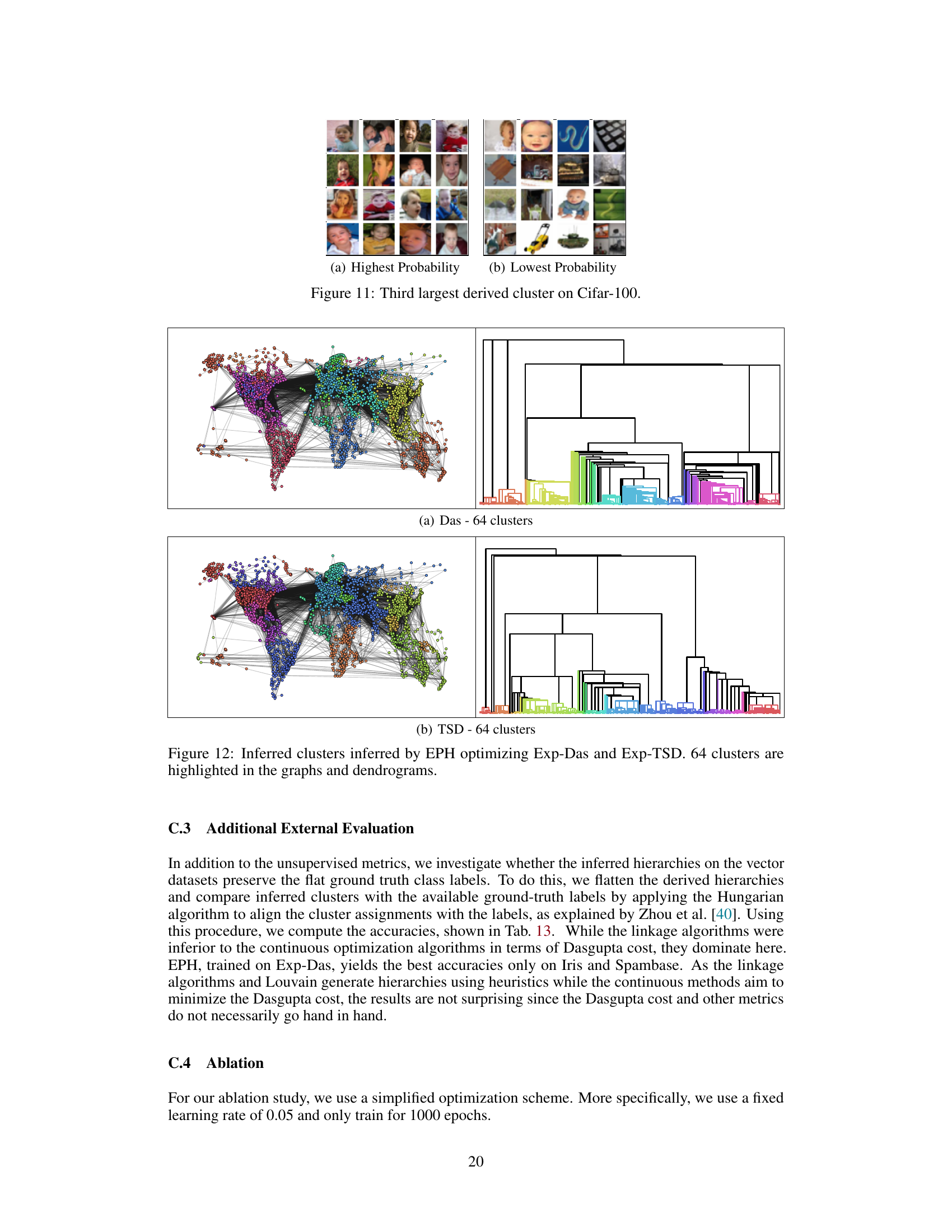
The figure shows the largest cluster inferred on the Cifar-100 dataset using EPH. The left subplot shows the 16 images with the highest probability, and the right subplot shows the 16 images with the lowest probability. The images with high probabilities are all similar and related to insects, demonstrating EPH’s ability to group similar images together. The images with low probabilities do not fit into the group, illustrating EPH’s capacity to measure uncertainty in cluster assignments.
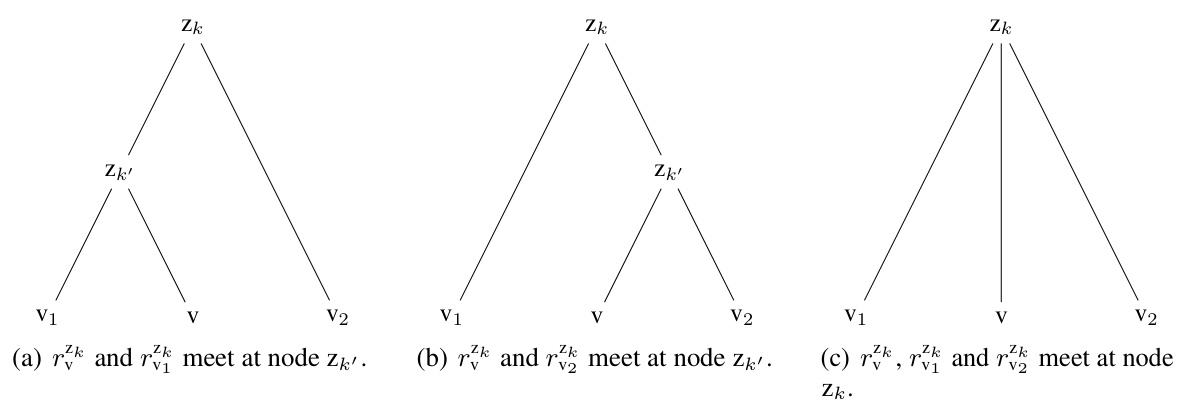
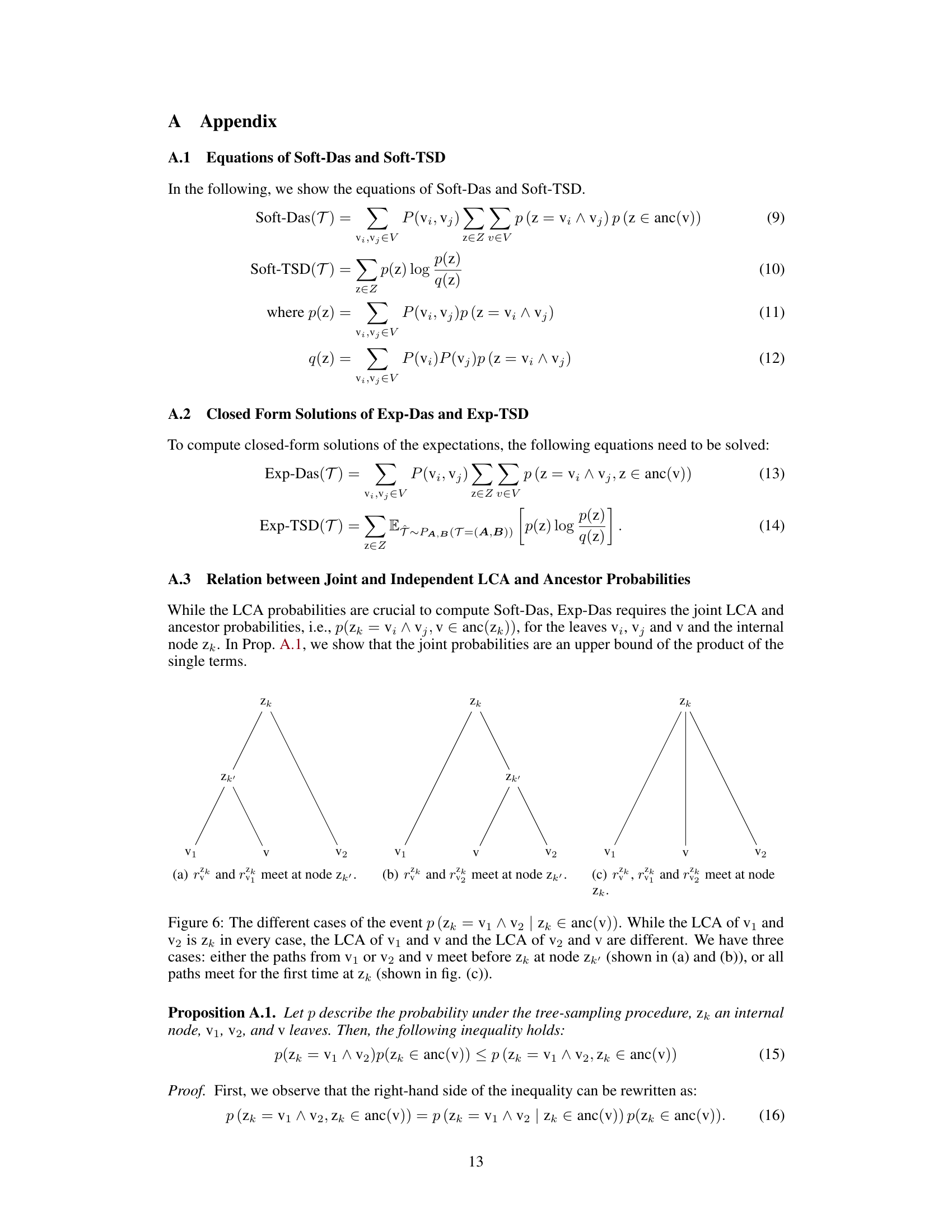
This figure illustrates the three possible scenarios when calculating the joint probability of the lowest common ancestor (LCA) and ancestor probabilities. It shows how the paths from three leaves (v1, v2, and v) to an internal node (zk) can intersect at different points (zk’, zk, or zk) depending on the tree structure. This is important for calculating the expected Dasgupta cost.
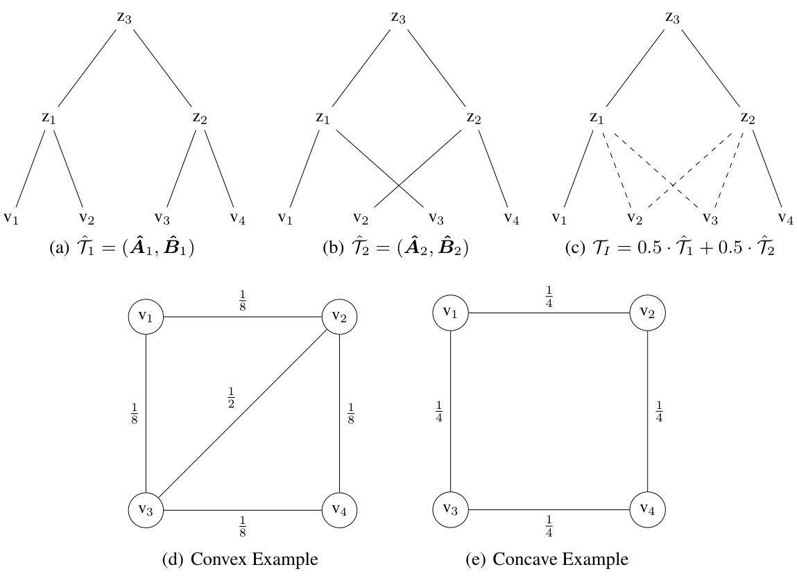
This figure demonstrates that the expected Dasgupta cost (Exp-Das), a function used in the Expected Probabilistic Hierarchies (EPH) method, is neither convex nor concave. It presents three different hierarchies (a, b, c) and two graphs (d, e). Hierarchy (c) is a linear interpolation between (a) and (b). Graphs (d) and (e) illustrate scenarios where the function behaves convexly and concavely, respectively. This non-convexity and non-concavity property complicates optimization but is explained and addressed within the EPH method.

This figure shows an example where the Flexible Probabilistic Hierarchy (FPH) method fails to find the optimal hierarchy that minimizes the Dasgupta cost. FPH’s continuous relaxation results in a Soft-Das score lower than the optimal discrete Dasgupta cost. In contrast, the Expected Probabilistic Hierarchies (EPH) method successfully finds the minimizing hierarchy. The figure uses an unweighted K4 graph for simplicity, but a similar issue is demonstrated with a weighted graph in Figure 8.

The figure visualizes the largest cluster inferred on the Cifar-100 dataset using the EPH method. It shows the 16 images with the highest probability (left) and the 16 images with the lowest probability (right) for the largest cluster. The images with high probabilities are visually similar (insects), demonstrating EPH’s ability to group similar images. The images with low probabilities do not visually fit in this group, illustrating EPH’s capability to measure uncertainty in cluster assignments.

The figure shows the largest cluster obtained by applying the EPH model on the Cifar-100 dataset. It displays two sets of 16 images each. (a) shows the 16 images with the highest probability of belonging to the cluster, and (b) shows the 16 images with the lowest probability. The images in (a) are visually similar and consistent with the theme of the cluster, whereas the images in (b) are more diverse and less representative of the cluster’s characteristics. This visualization demonstrates the capacity of EPH to both identify coherent clusters and quantify the uncertainty associated with cluster assignments.
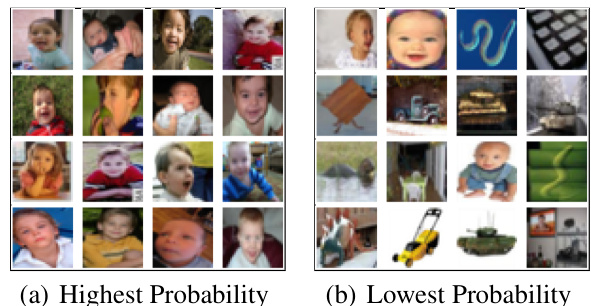
This figure visualizes the largest cluster identified by the EPH model on the Cifar-100 dataset. It showcases two sub-figures. (a) Highest Probability displays the 16 images with the highest probability within that cluster, showing a clear visual similarity related to insects. (b) Lowest Probability shows the 16 images with the lowest probability in that same cluster, demonstrating that they visually differ and do not strongly fit the identified theme. The images illustrate the model’s ability to discern clear visual patterns and quantify uncertainty within clusters by examining the probability assignments to each image.
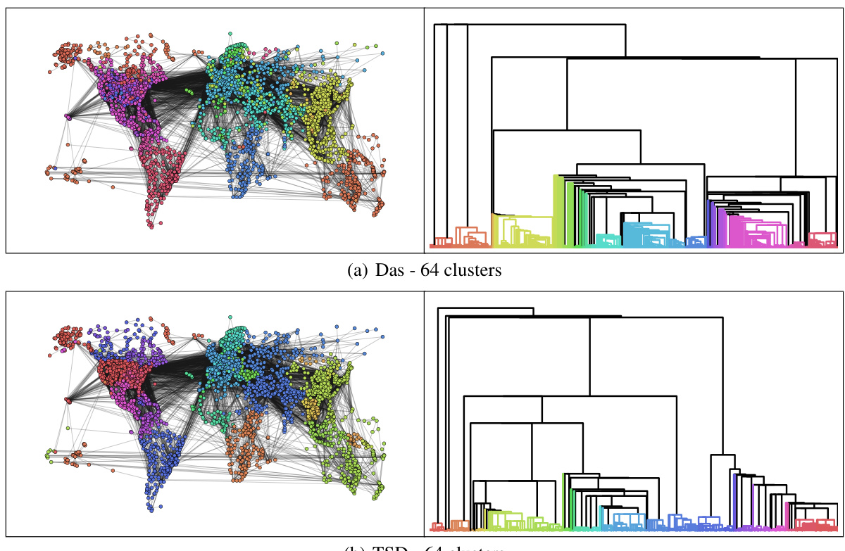
This figure visualizes the results of applying the Expected Probabilistic Hierarchies (EPH) method to the OpenFlight dataset, a graph representing flight connections between various locations worldwide. The left side shows the geographical distribution of the 64 clusters identified by EPH using two different objective functions: Exp-Das (expected Dasgupta cost) and Exp-TSD (expected Tree-Sampling Divergence). The right side displays the corresponding dendrograms for both objective functions, visually representing the hierarchical structure of the clusters. This allows for a direct comparison of the clustering results based on these two different metrics, showcasing how the hierarchical structure changes when optimizing for different objective functions. Each color represents a cluster, and the dendrogram’s branch lengths reflect the distance between clusters.

This figure visualizes the results of the EPH algorithm on five vector datasets (Zoo, Iris, Digits, Segmentation, and Spambase). It uses t-SNE to reduce the dimensionality of the data for better visualization. For each dataset, it shows three plots side-by-side: 1. Ground Truth Clusters: Shows the actual cluster assignments for each data point, providing a baseline for comparison. 2. Inferred Flattened Clusters: Shows the cluster assignments generated by the EPH algorithm after flattening the hierarchical structure. 3. Dendrograms: Provides a visual representation of the hierarchical clustering produced by EPH. The dendrogram illustrates the relationships between clusters and how they merge at different levels of granularity. The purpose is to allow a visual comparison of the ground truth and the EPH’s performance in clustering these datasets.

This figure displays the results of a linear interpolation experiment conducted on seven different graph datasets (Brain, Citeseer, Cora-ML, Genes, OpenFlight, Polblogs, and WikiPhysics). The experiment interpolates between the average linkage hierarchy and the hierarchy inferred by the Exp-Das algorithm, evaluating the Soft-Das and Exp-Das scores at different interpolation points (denoted by ‘Factor a’ on the x-axis). The y-axis shows the normalized Soft-Das and Exp-Das scores, respectively. This visualization provides insight into the relationship between the average linkage approach and the Exp-Das optimized hierarchy, highlighting potential differences in scoring metrics and the impact of the optimization procedure.

This figure shows the results of a hyperparameter study for the EPH model, investigating the impact of the number of sampled hierarchies and the number of sampled edges on the normalized Dasgupta cost. The left panel displays the effect of varying the number of sampled hierarchies, comparing EPH’s performance with the average linkage algorithm (AL) and training on the full graph. The right panel shows a similar comparison using different numbers of sampled edges. In both panels, the results are normalized across different datasets to allow for a clear comparison.

This figure shows the results of a hyperparameter study conducted to determine the optimal number of sampled hierarchies and edges for the EPH model. The left panel shows how the normalized Dasgupta cost varies with the number of sampled hierarchies for different datasets (Brain, OpenFlight, Genes, Citeseer, Cora-ML, Polblogs, WikiPhysics). The right panel shows how the normalized Dasgupta cost varies with the number of sampled edges for different datasets (Zoo, Iris, Glass, Digits, Segmentation, Spambase, Letter, Cifar-100). The average linkage algorithm (AL) and a training on the full graph (FG) are also included as baselines for comparison. The scores are normalized to have a mean of zero and a standard deviation of one for each dataset.

This figure provides a visual overview of the Expected Probabilistic Hierarchies (EPH) model. It shows the process of sampling discrete hierarchies and subgraphs, computing the expected scores, and updating the probabilistic hierarchy through backpropagation. The figure highlights the key steps involved in EPH and shows how differentiable hierarchy and subgraph sampling are used to optimize expected scores.

This figure illustrates the workflow of the Expected Probabilistic Hierarchies (EPH) model. EPH begins by sampling discrete hierarchies and subgraphs from the input data using differentiable sampling techniques. These samples are then used to compute and average the expected scores. Finally, backpropagation is used to update the probabilistic hierarchy, improving its ability to represent the underlying data structure.
More on tables

This table presents the results of different hierarchical clustering methods on various graph datasets. The methods are compared using two metrics: Dasgupta cost and Tree-sampling divergence. Lower Dasgupta cost and higher Tree-sampling divergence indicate better clustering performance. The table highlights the best performing method for each dataset and metric.
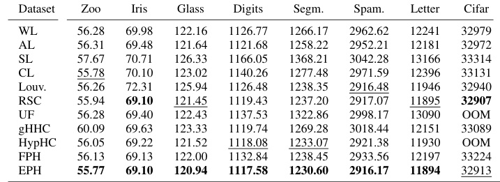
This table presents the Dasgupta costs achieved by different hierarchical clustering methods on eight vector datasets. The Dasgupta cost is a metric used to evaluate the quality of hierarchical clustering results. Lower scores indicate better clustering performance. The table compares several methods, including traditional linkage-based algorithms (WL, AL, SL, CL), and more recent methods like Louvain, RSC, UF, gHHC, HypHC, FPH, and the proposed method EPH. The best and second-best results for each dataset are highlighted in bold and underlined, respectively, to show the relative performance of each method.

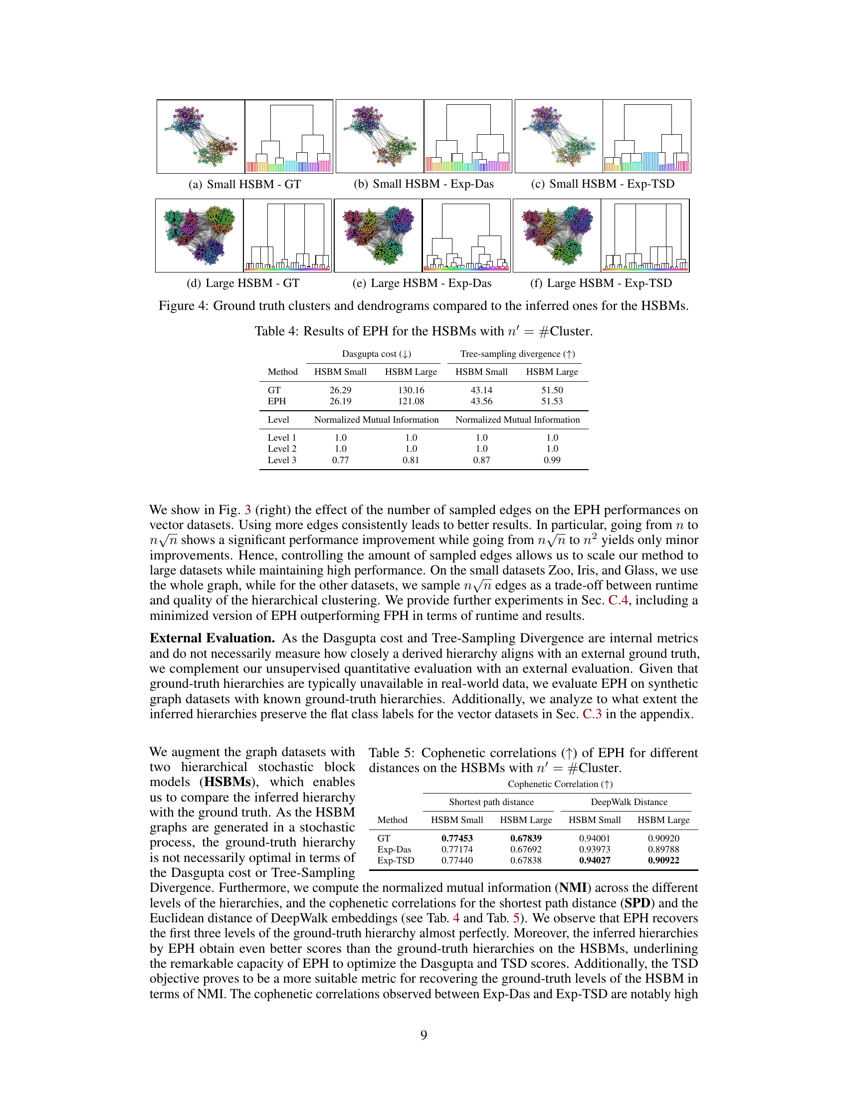
This table presents the results of the Expected Probabilistic Hierarchies (EPH) method on two Hierarchical Stochastic Block Models (HSBMs) with varying sizes. It compares the Dasgupta cost and Tree-sampling divergence of the hierarchies generated by EPH against the ground truth (GT) hierarchies. It also shows the normalized mutual information (NMI) at different levels of the hierarchy, indicating the alignment between the EPH-generated hierarchies and the ground truth.

This table presents the results of the Expected Probabilistic Hierarchies (EPH) method on two Hierarchical Stochastic Block Models (HSBMs), one small and one large. It compares the performance of EPH against the ground truth (GT) in terms of Dasgupta cost and Tree-Sampling Divergence. The normalized mutual information (NMI) at different levels of the hierarchy is also included, showing how well EPH recovers the structure of the ground truth HSBMs.

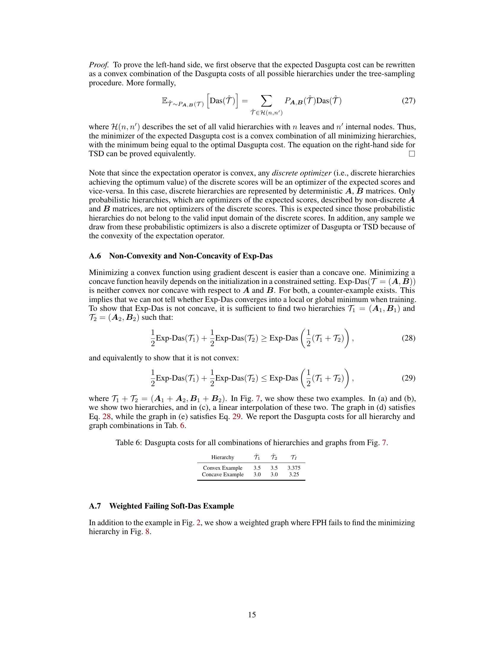
This table shows the Dasgupta costs for different combinations of hierarchies (T1, T2, and T_I) and graphs (convex and concave examples) from Figure 7 in the paper. The values demonstrate that the Exp-Das function is neither convex nor concave, supporting the paper’s claim about the function’s properties.
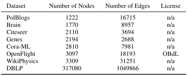
This table provides a summary of the graph datasets used in the paper’s experiments. For each dataset, it lists the number of nodes (vertices), the number of edges, and the license under which the dataset is available.

This table presents an overview of the eight vector datasets used in the paper’s experiments. For each dataset, it lists the number of data points, the number of attributes (features) for each data point, the number of classes, and the license under which the dataset is available. The datasets include Zoo, Iris, Glass, Digits, Segmentation, Spambase, Letter, and Cifar-100, representing a variety of data types and sizes.

This table presents a summary of the characteristics of the two hierarchical stochastic block models (HSBMs) used in the experiments. It shows the number of nodes, edges, and clusters for both the small and large HSBMs.
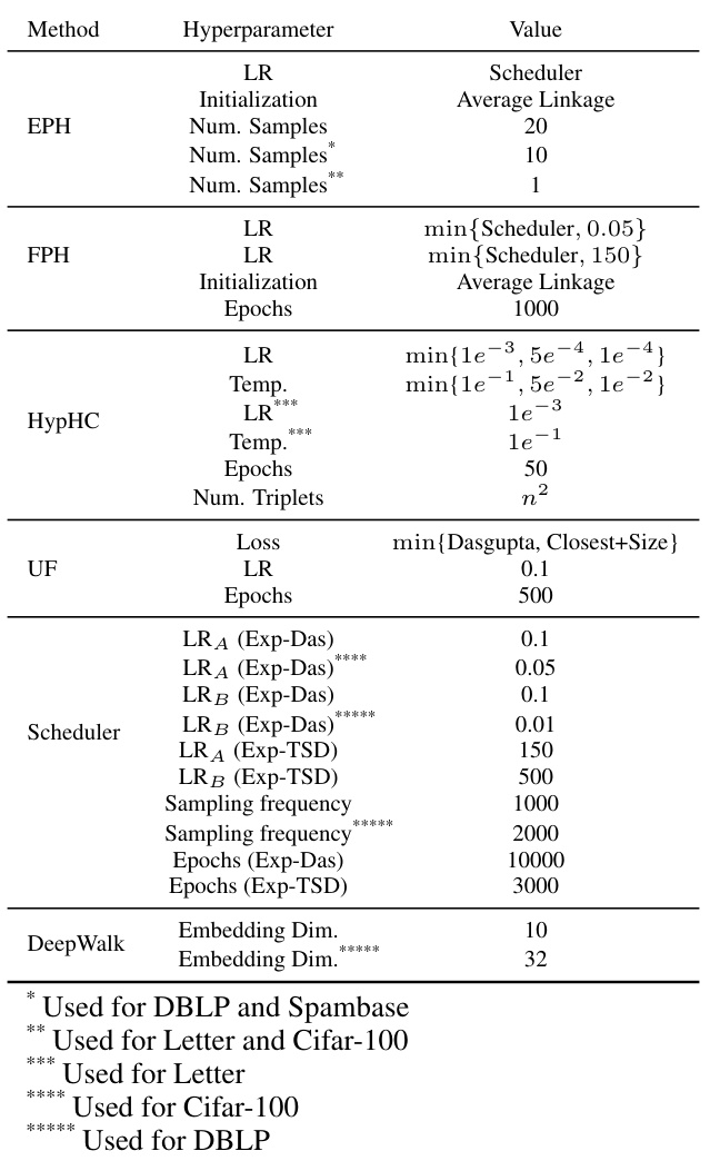
This table presents the hyperparameters used in the experiments for the different methods: EPH, FPH, HypHC, UF, and DeepWalk. It specifies the learning rate (LR), initialization methods, number of samples used for approximating expectations, temperature parameters for softmax functions, number of epochs for training, number of triplets, loss functions, and embedding dimensions. Specific hyperparameter settings are noted for different datasets (DBLP, Spambase, Letter, and Cifar-100) reflecting adaptations to variations in dataset properties.

This table presents the results of different hierarchical clustering methods on various graph datasets. The methods are compared based on two metrics: Dasgupta cost and Tree-sampling divergence. Lower Dasgupta cost and higher Tree-sampling divergence indicate better clustering performance. The table shows that the proposed EPH method achieves the best results in most cases, outperforming various baselines including other state-of-the-art methods.

This table presents the results obtained using the Flexible Probabilistic Hierarchy (FPH) method on two synthetic datasets generated using the Hierarchical Stochastic Block Model (HSBM): a small HSBM and a large HSBM. The results are evaluated based on two metrics: the Dasgupta cost and the Tree-sampling divergence. The table also includes the normalized mutual information (NMI) at different levels (Level 1, 2, and 3) of the hierarchy. The ground truth (GT) values are provided for comparison, allowing for the assessment of FPH’s ability to recover the ground truth hierarchy.

This table presents the Dasgupta costs achieved by different hierarchical clustering methods on eight vector datasets. The Dasgupta cost is a lower score is better metric used to evaluate the quality of a hierarchical clustering. The table compares the performance of various methods including traditional linkage algorithms (WL, AL, SL, CL), Louvain modularity maximization, recursive sparsest cut, and more recent continuous methods such as Ultrametric Fitting, Hyperbolic Hierarchical Clustering, gradient-based Hyperbolic Hierarchical Clustering, Flexible Probabilistic Hierarchy, and the proposed Expected Probabilistic Hierarchies (EPH) method. The best and second-best scores for each dataset are highlighted.

This table compares the Dasgupta costs achieved by using constrained and unconstrained optimization methods on various graph datasets. The number of internal nodes (n’) is fixed at 512. The results highlight the impact of enforcing the row-stochasticity constraint on the optimization process, revealing how this constraint affects the quality of the resulting hierarchical clustering as measured by the Dasgupta cost.

This table compares the Dasgupta costs obtained using different initialization methods for the EPH model on several graph datasets. The first three rows show the initial Dasgupta costs before training using random, Average Linkage (AL), and Flexible Probabilistic Hierarchy (FPH) methods. The last three rows present the Dasgupta costs after training with the EPH model using each of these initialization methods. The best and second-best results are highlighted in bold and underlined, respectively.

This table compares the Dasgupta costs achieved by using direct parametrization versus embedding parametrization for the matrices A and B in the EPH model. It shows that the direct parametrization consistently outperforms the embedding approach except for PolBlogs. The results highlight the trade-off between the simplicity and performance of the direct method compared to the added complexity of embedding, especially when considering that the embedding approach required significantly more training epochs (20000 vs 1000).

This table presents the results of different hierarchical clustering methods on various graph datasets. The methods compared include several linkage algorithms (WL, AL), Louvain, recursive sparsest cut (RSC), Ultrametric Fitting (UF), gradient-based Hyperbolic Hierarchical Clustering (gHHC), Hyperbolic Hierarchical Clustering (HypHC), Flexible Probabilistic Hierarchy (FPH), and the proposed Expected Probabilistic Hierarchies (EPH). The table shows the Dasgupta cost and Tree-sampling divergence for each method on each dataset. Lower Dasgupta cost and higher Tree-sampling divergence indicate better performance.

This table presents the standard deviations of the Dasgupta cost and tree-sampling divergence for different graph datasets. The values represent the variability or uncertainty in the results obtained for the different algorithms on each dataset. A higher standard deviation indicates more variability in the results.

This table presents a comparison of the Dasgupta cost achieved by different hierarchical clustering methods on eight vector datasets. The Dasgupta cost is a lower-is-better metric that evaluates the quality of a hierarchical clustering. The table shows that EPH consistently achieves the lowest Dasgupta cost across most datasets, indicating superior performance compared to other methods.
This table presents a comparison of different hierarchical clustering methods on several graph datasets. The methods compared include various linkage algorithms (WL, AL, Louv, RSC), continuous optimization approaches (UF, gHHC, HypHC, FPH), and the proposed EPH method. For each method and each dataset, the Dasgupta cost and tree-sampling divergence are reported. The best-performing method for each metric and dataset is shown in bold, with the second-best underlined. This allows for a quantitative comparison of the methods across different datasets and metrics.

This table presents a comparison of different hierarchical clustering methods on several graph datasets. The methods are evaluated based on two metrics: Dasgupta cost (lower is better) and Tree-sampling divergence (higher is better). The table shows the performance of various methods (WL, AL, Louv, RSC, UF, gHHC, HypHC, FPH, and EPH) across multiple datasets (PolBlogs, Brain, Citeseer, Genes, Cora-ML, OpenFlight, WikiPhysics, and DBLP). The best and second-best performing methods for each dataset and metric are highlighted.

This table presents the results of different hierarchical clustering methods on several graph datasets. It shows the Dasgupta cost and Tree-sampling divergence scores for each method. The best-performing method for each dataset and metric is highlighted in bold, while the second-best is underlined. This allows for a comparison of the performance of various algorithms across different datasets and metrics.

This table shows the runtime in seconds for various hierarchical clustering algorithms on eight different graph datasets. The number of internal nodes (n’) is fixed at 512. The algorithms include standard linkage methods (WL, AL, Louv.), a recursive sparsest cut method (RSC), gradient-based continuous methods (UF, gHHC, HypHC), the Flexible Probabilistic Hierarchy method (FPH), and the proposed Expected Probabilistic Hierarchies method (EPH) and its minimized version. The table helps illustrate the computational efficiency of the different methods, particularly highlighting the runtime of EPH compared to others.
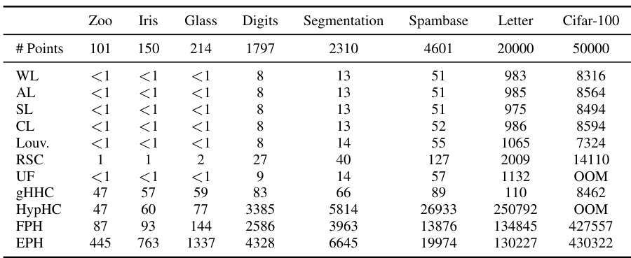
This table shows the runtime in seconds for different hierarchical clustering algorithms on eight vector datasets. The number of internal nodes (n’) used in the algorithms is the minimum between n-1 (where n is the number of data points in the dataset) and 512. The algorithms compared include various linkage methods (WL, AL, SL, CL), Louvain, RSC, UF, gHHC, HypHC, FPH, and EPH. The table provides a detailed comparison of the computational efficiency of each algorithm on various datasets of different sizes.
Full paper#
