TL;DR#
Traditional time series forecasting methods often struggle with variable-length data and require separate model training for different prediction horizons. Recent attempts to use Large Language Models (LLMs) have been hindered by the mismatch between LLMs’ inherent autoregressive nature and the common non-autoregressive approaches used in time series forecasting. This leads to inefficient use of LLM capabilities and often results in lower generalization performance.
AutoTimes directly addresses these issues. It introduces a novel method that fully leverages LLMs’ autoregressive properties to forecast time series of arbitrary lengths. By representing time series as prompts and incorporating contextual information, AutoTimes achieves state-of-the-art accuracy with only 0.1% trainable parameters and a significant speedup in training and inference compared to other LLM-based approaches. This method exhibits flexibility in handling variable-length lookback windows and scales well with larger LLMs, opening up exciting new possibilities for time series forecasting and foundation model development.
Key Takeaways#
Why does it matter?#
This paper is crucial for researchers in time series forecasting because it demonstrates the effectiveness of adapting large language models (LLMs) for this task. It introduces a novel autoregressive approach, surpassing previous methods in accuracy and efficiency. This opens new avenues for research exploring LLM applications in other sequential data domains and developing foundation models for time series analysis.
Visual Insights#

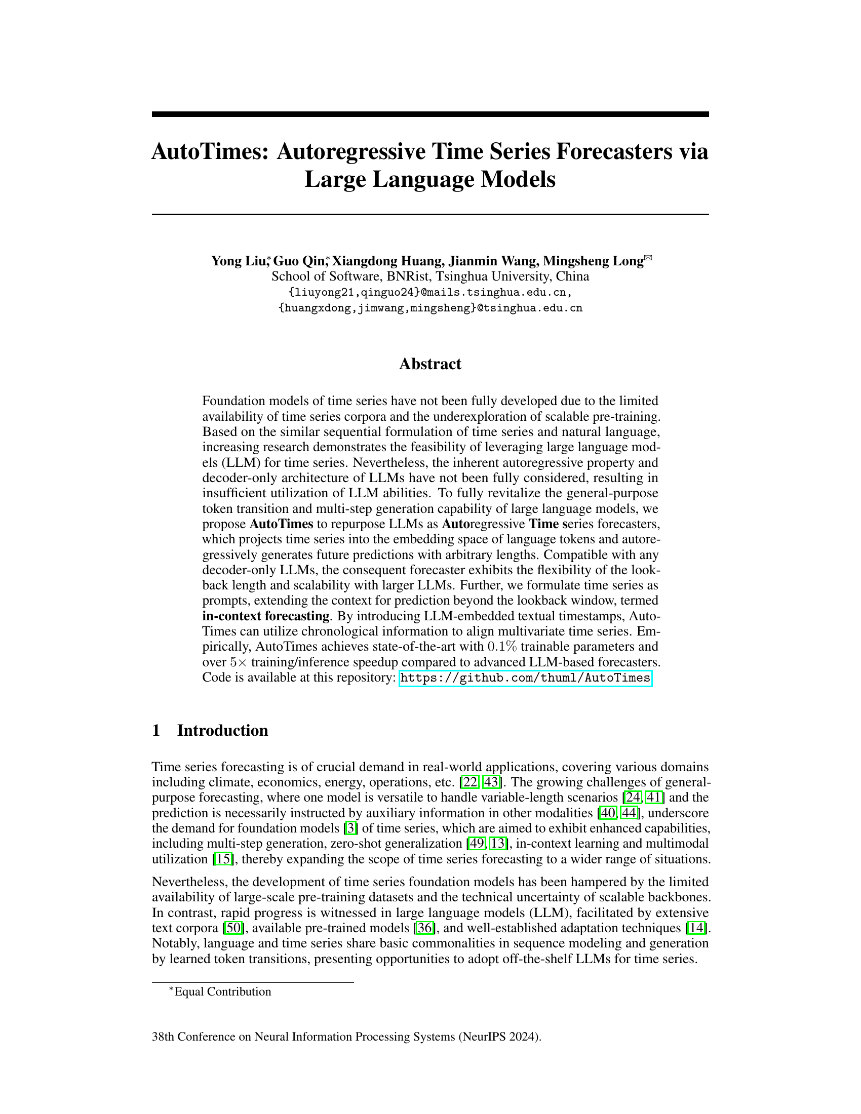
🔼 This figure compares two approaches for using LLMs in time series forecasting. (a) shows the prevalent non-autoregressive approach, where the LLM processes a flattened representation of the lookback series to generate predictions all at once. In contrast, the figure highlights the autoregressive approach proposed in the paper. This approach leverages the inherent autoregressive nature of LLMs for sequential prediction of the next token in the series. (b) demonstrates a comparison of prompting mechanisms. The traditional method uses natural language prompts, which can introduce modality disparities. The proposed method leverages time series itself for prompting, a technique referred to as ‘in-context forecasting’.
read the caption
Figure 1: (a) Prevalent LLM4TS methods non-autoregressively generate predictions with the globally flattened representation of lookback series, while large language models inherently predict the next tokens by autoregression [47]. (b) Previous methods adopt language prompts that may lead to the modality disparity, while we find time series can be self-prompted, termed in-context forecasting.

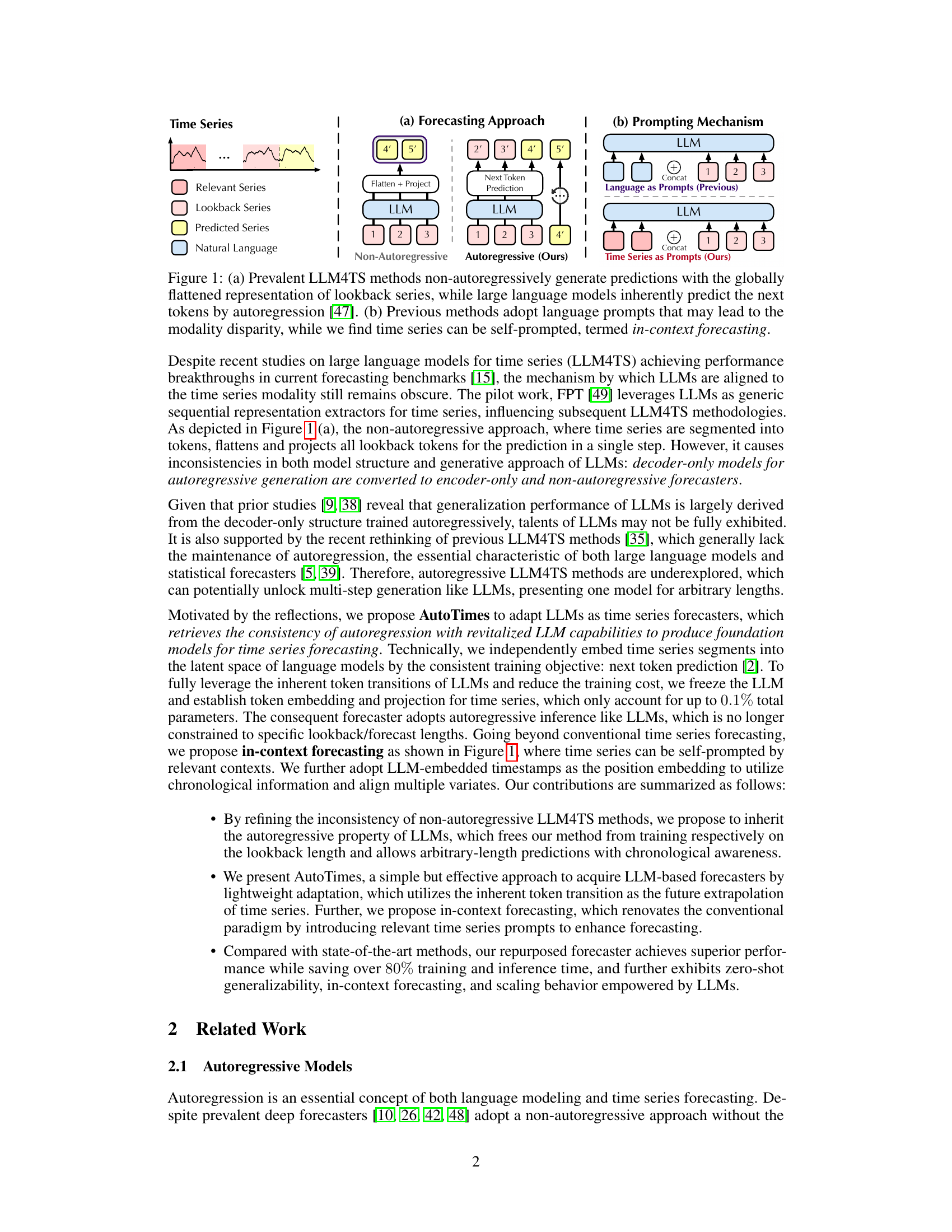
🔼 This table compares several Large Language Model for Time Series (LLM4TS) methods based on three key aspects: whether they are autoregressive, whether they freeze the pre-trained Large Language Model (LLM), and whether they are multimodal. Autoregressive models generate predictions sequentially, using previous predictions to inform current ones. Freezing the LLM means that only a small set of parameters are trained, reducing computational cost. Multimodal methods incorporate data from sources other than just the time series, like textual descriptions or images. The table highlights that AutoTimes is unique in combining all three of these characteristics.
read the caption
Table 1: Comparison of LLM4TS methods: Autoregressive categorizes LLM-based forecasters by whether to conduct autoregression. Freeze LLM enables quick adaptation, which would otherwise require significant resources for fine-tuning. Multimodal refers to the utilization of information from other modalities. Prior to AutoTimes, none of the LLM4TS methods achieved all three.
In-depth insights#
LLM4TS Autoregression#
LLM4TS (Large Language Models for Time Series) research has predominantly focused on non-autoregressive methods, treating LLMs as feature extractors rather than leveraging their inherent autoregressive capabilities for sequential prediction. Autoregressive approaches are crucial because they directly align with the nature of time series data and the strength of LLMs in generating sequential outputs. By fully utilizing the autoregressive property of LLMs, models can naturally generate multi-step predictions with arbitrary lengths, overcoming limitations of non-autoregressive methods that often require separate models for different forecast horizons. This inherent autoregressive nature offers significant advantages, enabling more efficient and accurate forecasting, especially for longer prediction windows where error accumulation in non-autoregressive methods becomes a significant problem. Furthermore, autoregressive LLM4TS models may also improve zero-shot generalization, as the autoregressive training better captures the underlying sequential patterns in time series, leading to more robust models capable of handling unseen data.
In-context Forecasting#
The concept of “In-context Forecasting” presented in the research paper proposes a novel approach to leverage the capabilities of Large Language Models (LLMs) for time series forecasting. It suggests that instead of solely relying on a limited lookback window of time series data, the model’s prediction context can be significantly enriched by incorporating relevant prior time series data as prompts. This method, termed “self-prompting,” enhances forecasting accuracy by effectively extending the context beyond the immediate lookback period. The key advantage lies in the model’s ability to learn from broader contextual patterns and dependencies, thereby potentially improving forecasting accuracy and robustness. The paper further investigates the strategic selection of these prompts, exploring the impact of chronological ordering and the use of LLM-embedded timestamps to align multiple time series and maximize the benefits of this approach. This innovation has the potential to significantly improve forecasting capabilities of LLMs in various applications by allowing for better context awareness and generalization to unseen data.
Multi-variate Time Series#
Analyzing multivariate time series presents unique challenges and opportunities. The inherent complexity arises from the interdependencies between multiple variables, requiring sophisticated models to capture these relationships effectively. Traditional univariate methods often fail to account for these interactions, leading to inaccurate predictions. Therefore, techniques designed specifically for multivariate data are essential, often involving vector autoregressive models (VAR) or dynamic factor models. The selection of an appropriate model depends on the characteristics of the data, such as stationarity, autocorrelation, and the presence of non-linear relationships. Dimensionality reduction techniques can be beneficial when dealing with high-dimensional data, helping manage computational complexity and improving model interpretability. Forecasting accuracy in multivariate scenarios is critically important for decision-making across numerous fields, including finance, environmental science, and healthcare, impacting resource allocation, risk management, and policy decisions. Advanced machine learning techniques, like deep learning, also show promise in tackling the complexities of multivariate time series analysis.
LLM Adaptation#
LLM adaptation in time series forecasting involves leveraging pre-trained large language models (LLMs) for the task. A crucial aspect is how the LLM is adapted to handle the sequential nature of time series data effectively. Common approaches include fine-tuning the LLM on a time series dataset, often adapting the input embedding layer to represent temporal data properly. However, this can be computationally expensive and may not fully exploit the LLM’s inherent capabilities. Alternative strategies focus on parameter-efficient fine-tuning techniques like LoRA (Low-Rank Adaptation), which freeze most of the LLM’s weights and only adjust a small set of parameters. Another key consideration is maintaining the autoregressive nature of the LLM, allowing it to generate predictions iteratively. This autoregressive approach, unlike some non-autoregressive methods, directly leverages the LLMs generative capacity. The choice of adaptation method significantly impacts the balance between model performance, training efficiency, and computational cost. Future research should explore more effective and efficient methods for LLM adaptation for enhanced accuracy and generalization in time series forecasting.
Future of LLM4TS#
The future of LLMs in time series forecasting (LLM4TS) is bright, but faces challenges. Autoregressive approaches, fully leveraging the inherent capabilities of LLMs, show great promise, surpassing non-autoregressive methods in accuracy and efficiency. In-context learning allows for better generalization and adaptation to unseen data, reducing the reliance on extensive fine-tuning. Multimodal approaches, integrating time series with other data types (text, images), will unlock new forecasting capabilities. However, addressing limitations in probabilistic forecasting, improving computational efficiency for very large LLMs, and ensuring fair and responsible use of these powerful models remain key research areas. Further exploration of low-rank adaptation techniques offers a path to reduce the computational burden and enhance the efficiency of LLM adaptation. Developing robust methods for prompt engineering and context selection is also crucial for maximizing the performance and reliability of LLM4TS models in real-world applications.
More visual insights#
More on figures

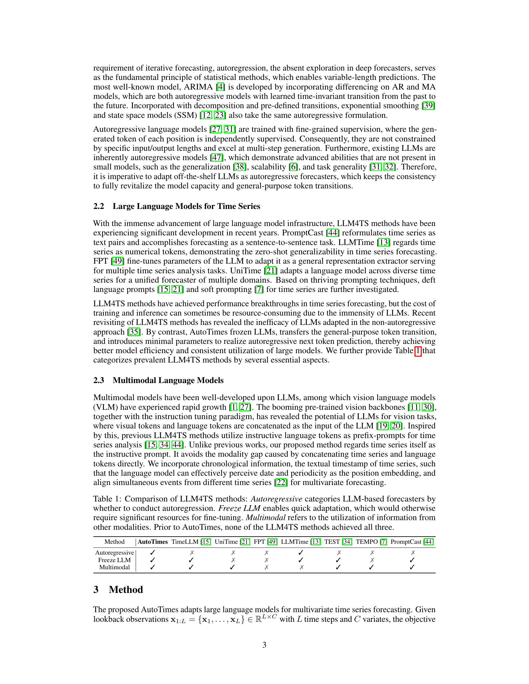
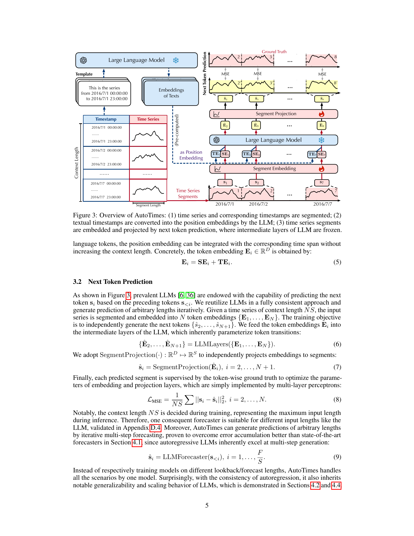
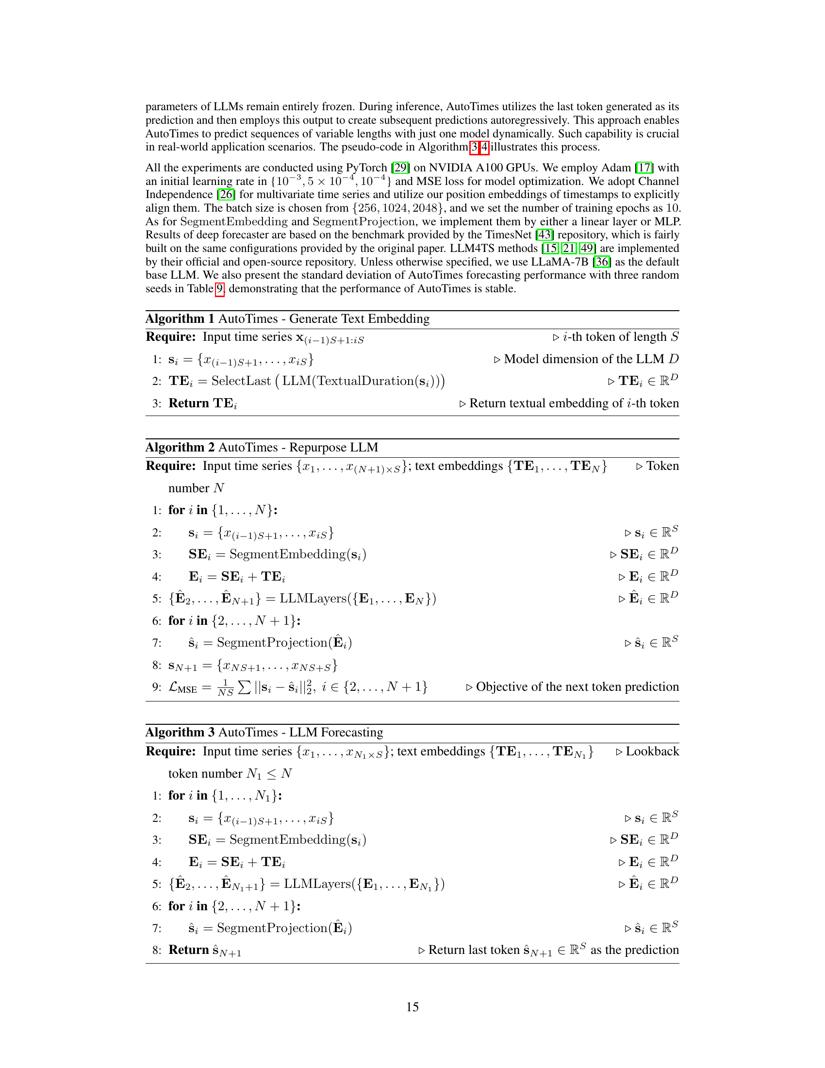
🔼 This figure illustrates the core idea of AutoTimes, which repurposes large language models (LLMs) for time series forecasting. It shows how a sequence of time series data points is converted into a sequence of tokens, similar to how words are tokens in natural language. The LLM, which is trained on natural language data, is then used to predict the next tokens in the time series sequence. The figure visually depicts the token-wise alignment between the time series tokens and the language tokens, showing that the LLM’s inherent autoregressive property (predicting the next token based on the previous ones) is leveraged for forecasting. The color gradient from dark to light indicates the flow of information, from the lookback window to the future predictions.
read the caption
Figure 2: An example to illustrate how AutoTimes adapts language models for time series forecasting.
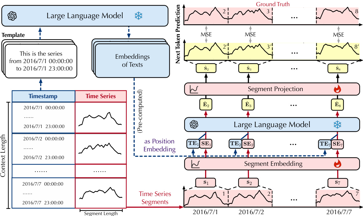
🔼 This figure illustrates the overall architecture of AutoTimes. It shows how time series data and timestamps are processed. First, the time series and timestamps are segmented into smaller chunks. Textual timestamps are then converted into position embeddings using a large language model (LLM). The time series segments are then embedded and projected using the LLM’s intermediate layers (the LLM weights are frozen during this process). Finally, next-token prediction is used for forecasting.
read the caption
Figure 3: Overview of AutoTimes: (1) time series and corresponding timestamps are segmented; (2) textual timestamps are converted into the position embeddings by the LLM; (3) time series segments are embedded and projected by next token prediction, where intermediate layers of LLM are frozen.

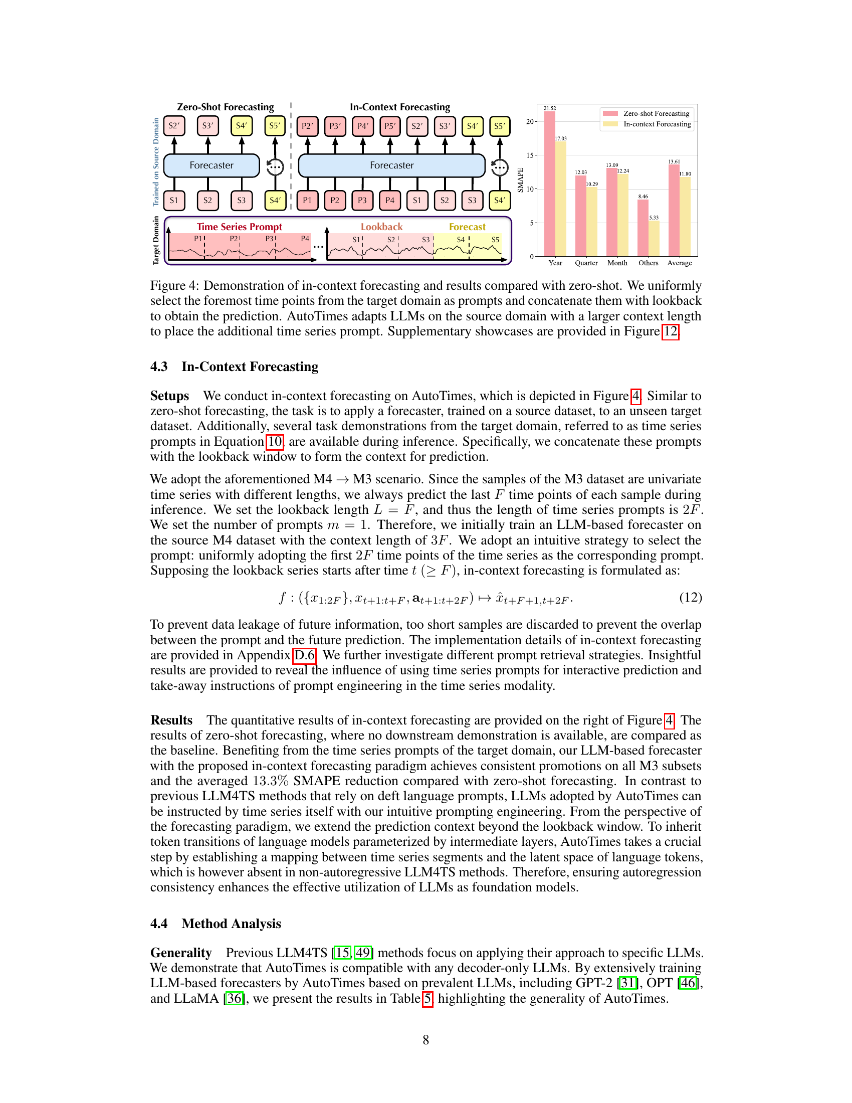
🔼 This figure demonstrates the in-context forecasting approach of AutoTimes and compares it with the zero-shot approach. In the zero-shot approach, the model trained on a source domain is directly applied to a target domain without any additional information. The in-context approach, however, incorporates additional time series prompts from the target domain as context. These prompts are concatenated with the lookback window before feeding into the forecaster. The bar chart visually compares the SMAPE (Symmetric Mean Absolute Percentage Error) results of both approaches across different data subsets (Year, Quarter, Month, Others), demonstrating the effectiveness of the in-context forecasting method.
read the caption
Figure 4: Demonstration of in-context forecasting and results compared with zero-shot. We uniformly select the foremost time points from the target domain as prompts and concatenate them with lookback to obtain the prediction. AutoTimes adapts LLMs on the source domain with a larger context length to place the additional time series prompt. Supplementary showcases are provided in Figure 12.
🔼 This figure illustrates the AutoTimes model architecture. The process begins by segmenting the input time series into smaller segments and representing timestamps as text. These textual timestamps are then processed by a large language model (LLM) to generate position embeddings. The time series segments are also embedded, and these embeddings are concatenated with the position embeddings. The resulting embeddings are then fed into the LLM for next token prediction, with the intermediate layers of the LLM frozen to reduce computational cost. The output is a prediction of future time series values.
read the caption
Figure 3: Overview of AutoTimes: (1) time series and corresponding timestamps are segmented; (2) textual timestamps are converted into the position embeddings by the LLM; (3) time series segments are embedded and projected by next token prediction, where intermediate layers of LLM are frozen.

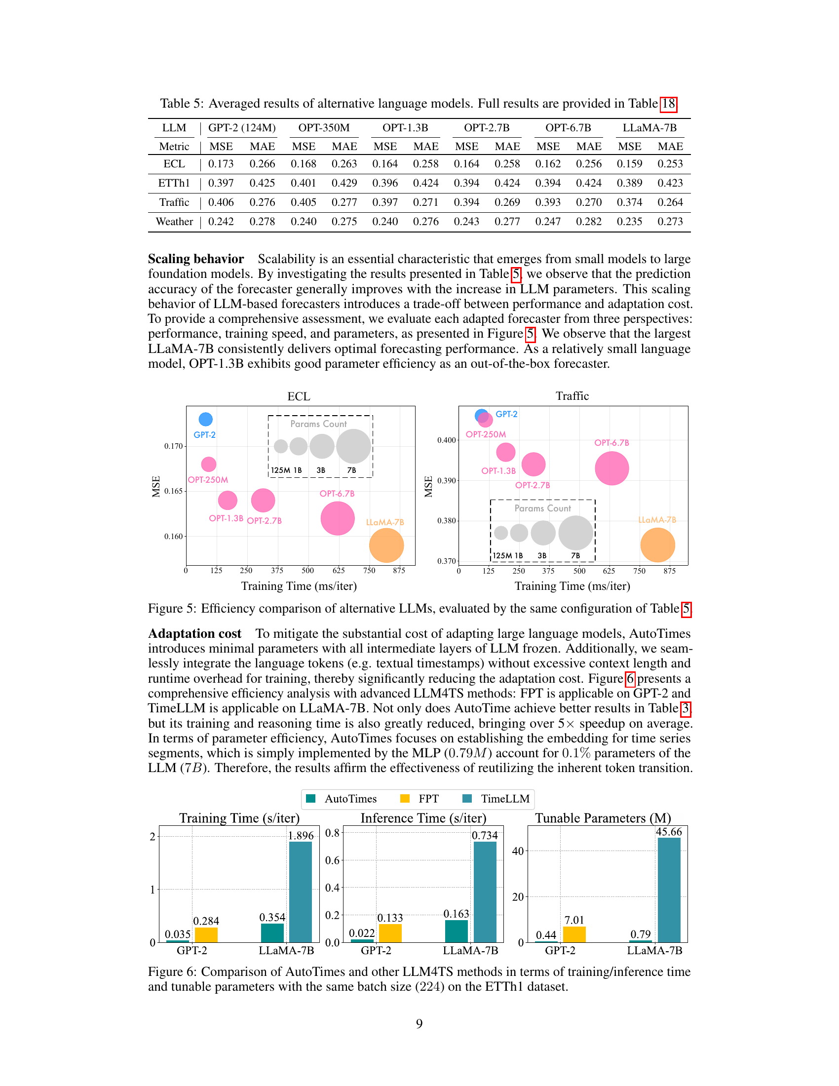
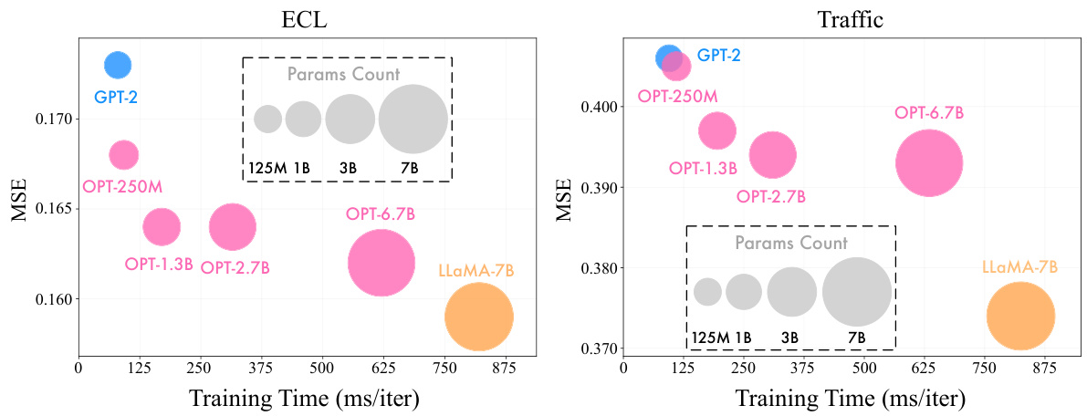
🔼 This figure compares the training time, inference time, and number of tunable parameters for different LLMs used in the AutoTimes model. The LLMs compared are GPT-2 and LLaMA-7B. The results show that AutoTimes is significantly more efficient in terms of training and inference time, and uses far fewer tunable parameters compared to other LLM-based forecasting methods. This highlights the efficiency of AutoTimes in leveraging LLMs for time-series forecasting.
read the caption
Figure 6: Efficiency comparison of alternative LLMs, evaluated by the same configuration of Table 5.

🔼 This figure illustrates the overall architecture of the AutoTimes model. It shows how the model processes time series data by segmenting it and converting timestamps into position embeddings using a pre-trained Large Language Model (LLM). The core idea is to embed time series segments into the LLM’s embedding space, leveraging its inherent capabilities for token transition and prediction. Importantly, the intermediate layers of the LLM are frozen, thus, the model efficiently uses the pre-trained LLM’s power without heavy training.
read the caption
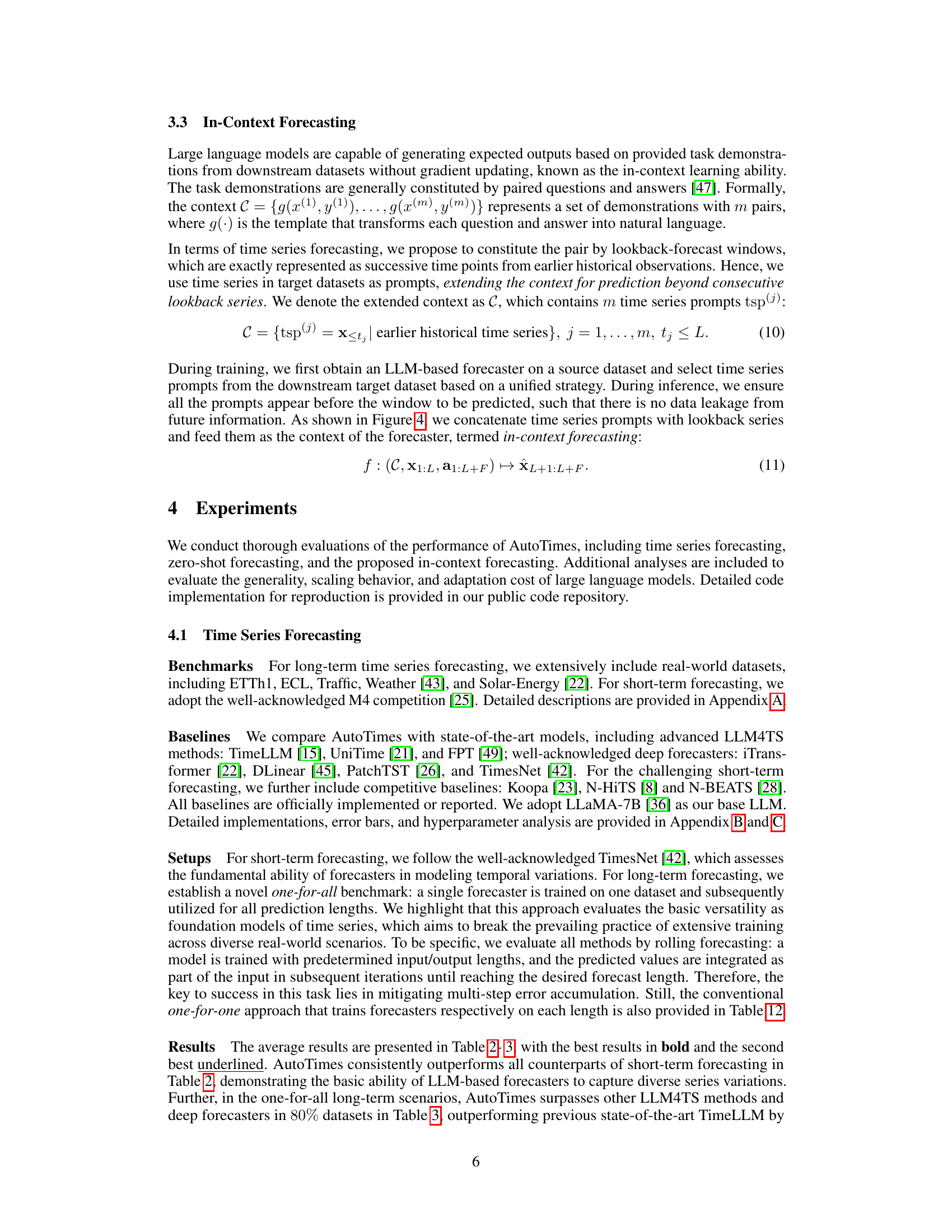
Figure 3: Overview of AutoTimes: (1) time series and corresponding timestamps are segmented; (2) textual timestamps are converted into the position embeddings by the LLM; (3) time series segments are embedded and projected by next token prediction, where intermediate layers of LLM are frozen. language tokens, the position embedding can be integrated with the corresponding time span without increasing the context length. Concretely, the token embedding Eᵢ ∈ RD is obtained by: Eᵢ = SEᵢ + TEᵢ.

🔼 This figure shows the impact of different hyperparameters on the performance of AutoTimes for various forecast lengths. The hyperparameters tested are the number of layers and the hidden dimension in both the Segment Embedding and Segment Projection components, the context length, and the segment length. Each line represents a different forecast length (pred-96, pred-192, pred-336, pred-720), and the x-axis shows the different values tested for each hyperparameter. The y-axis shows the Mean Squared Error (MSE). This allows for an assessment of how sensitive the model’s performance is to changes in these hyperparameters and helps in determining optimal settings.
read the caption
Figure 7: Hyperparameter sensitivity of AutoTimes. Each curve presents a specific forecast length.

🔼 This figure illustrates the AutoTimes model architecture. It shows how time series data and timestamps are processed. First, time series are segmented into smaller chunks and textual timestamps are created. Then, the LLM converts the timestamps into position embeddings. Next, time series segments are converted into embeddings using a segment embedding function, and these embeddings are then combined with the timestamp embeddings. Finally, next-token prediction is performed using the frozen layers of a pre-trained LLM. The resulting token embeddings form the input of subsequent layers in the model’s autoregressive process. The overall approach leverages pre-trained LLMs for forecasting with minimal training.
read the caption
Figure 3: Overview of AutoTimes: (1) time series and corresponding timestamps are segmented; (2) textual timestamps are converted into the position embeddings by the LLM; (3) time series segments are embedded and projected by next token prediction, where intermediate layers of LLM are frozen. language tokens, the position embedding can be integrated with the corresponding time span without increasing the context length. Concretely, the token embedding Eᵢ ∈ RD is obtained by: Eᵢ = SEᵢ + TEᵢ.

🔼 This figure compares two approaches for using LLMs for time series forecasting. (a) shows the common non-autoregressive approach where the LLM processes the entire lookback series at once to generate predictions. This is contrasted with (b), which shows the autoregressive approach used by AutoTimes. The key difference is AutoTimes uses an autoregressive approach to generate the next prediction token at a time, which is how LLMs naturally function. It also shows that AutoTimes uses a self-prompting mechanism (in-context forecasting) which differs from the use of language prompts in prior work.
read the caption
Figure 1: (a) Prevalent LLM4TS methods non-autoregressively generate predictions with the globally flattened representation of lookback series, while large language models inherently predict the next tokens by autoregression [47]. (b) Previous methods adopt language prompts that may lead to the modality disparity, while we find time series can be self-prompted, termed in-context forecasting.

🔼 This figure compares the prevalent large language model for time series forecasting methods. Panel (a) shows that most existing methods don’t use the autoregressive nature of LLMs, processing the entire lookback period at once rather than sequentially. Panel (b) highlights a key difference: the proposed method uses the time series itself as a prompt (in-context forecasting), avoiding issues that arise from using natural language prompts that don’t directly align with the time series data.
read the caption
Figure 1: (a) Prevalent LLM4TS methods non-autoregressively generate predictions with the globally flattened representation of lookback series, while large language models inherently predict the next tokens by autoregression [47]. (b) Previous methods adopt language prompts that may lead to the modality disparity, while we find time series can be self-prompted, termed in-context forecasting.
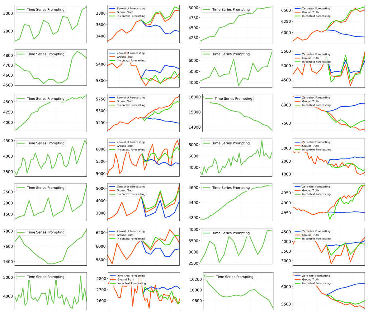
🔼 This figure demonstrates the results of in-context forecasting and compares them to zero-shot forecasting. In in-context forecasting, time series prompts from the target domain are concatenated with the lookback series before feeding to the model. The results show that using these prompts improves forecasting performance compared to the zero-shot approach. Supplementary figures showing additional results are referenced.
read the caption
Figure 4: Demonstration of in-context forecasting and results compared with zero-shot. We uniformly select the foremost time points from the target domain as prompts and concatenate them with lookback to obtain the prediction. AutoTimes adapts LLMs on the source domain with a larger context length to place the additional time series prompt. Supplementary showcases are provided in Figure 12.
More on tables

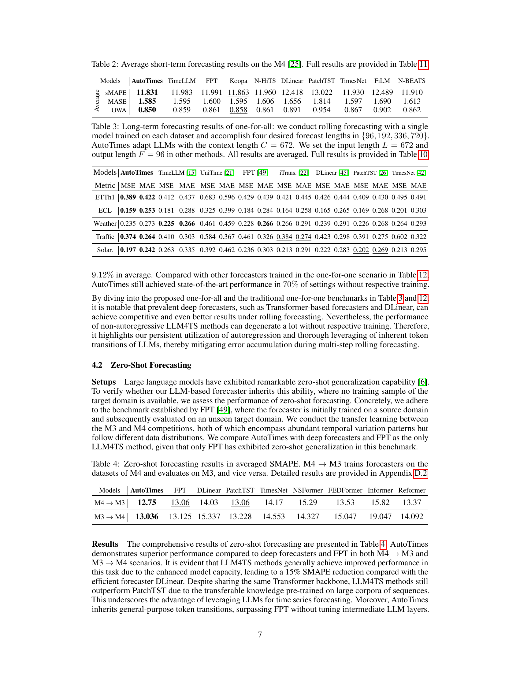
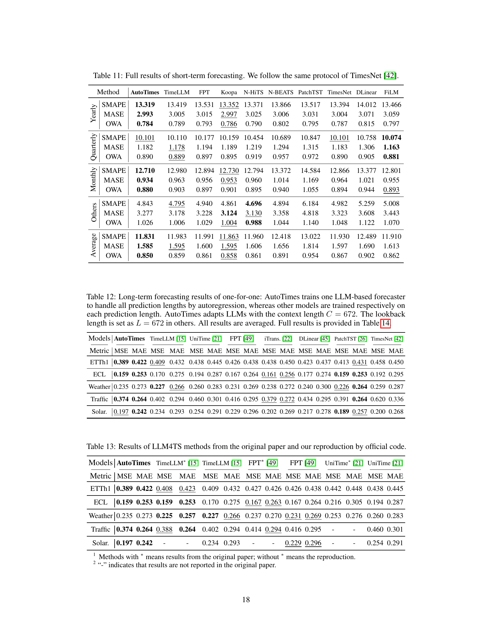
🔼 This table presents the average results of short-term time series forecasting on the M4 dataset. It compares the performance of AutoTimes against several other state-of-the-art methods, including TimeLLM, FPT, Koopa, N-HiTS, DLinear, PatchTST, TimesNet, FiLM, and N-BEATS. The metrics used for comparison are SMAPE (Symmetric Mean Absolute Percentage Error), MASE (Mean Absolute Scaled Error), and OWA (Overall Weighted Average). Detailed results for each method on each time series within the M4 dataset are available in Table 11.
read the caption
Table 2: Average short-term forecasting results on the M4 [25]. Full results are provided in Table 11.

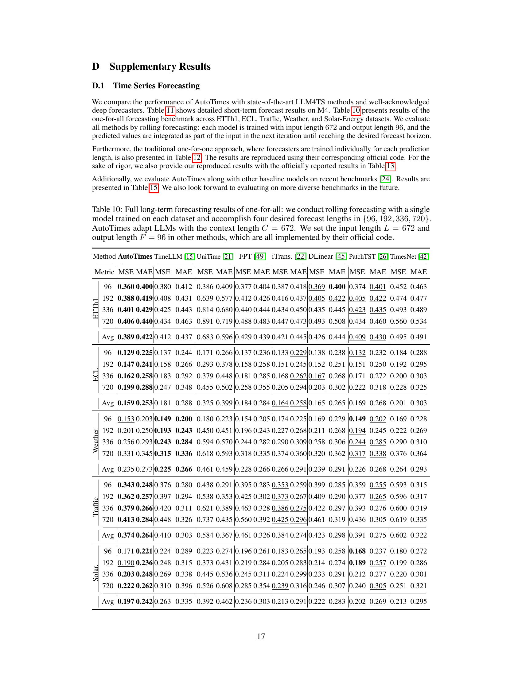
🔼 This table presents the results of long-term time series forecasting experiments using a ‘one-for-all’ approach. A single model is trained on each dataset and then used to generate forecasts of different lengths (96, 192, 336, and 720 time steps). The AutoTimes model uses a context length of 672 time steps, while other methods use an input length of 672 and an output length of 96. The table shows the average results across all forecast lengths, with more detailed results in Table 10.
read the caption
Table 3: Long-term forecasting results of one-for-all: we conduct rolling forecasting with a single model trained on each dataset and accomplish four desired forecast lengths in {96, 192, 336, 720}. AutoTimes adapt LLMs with the context length C = 672. We set the input length L = 672 and output length F = 96 in other methods. All results are averaged. Full results is provided in Table 10.

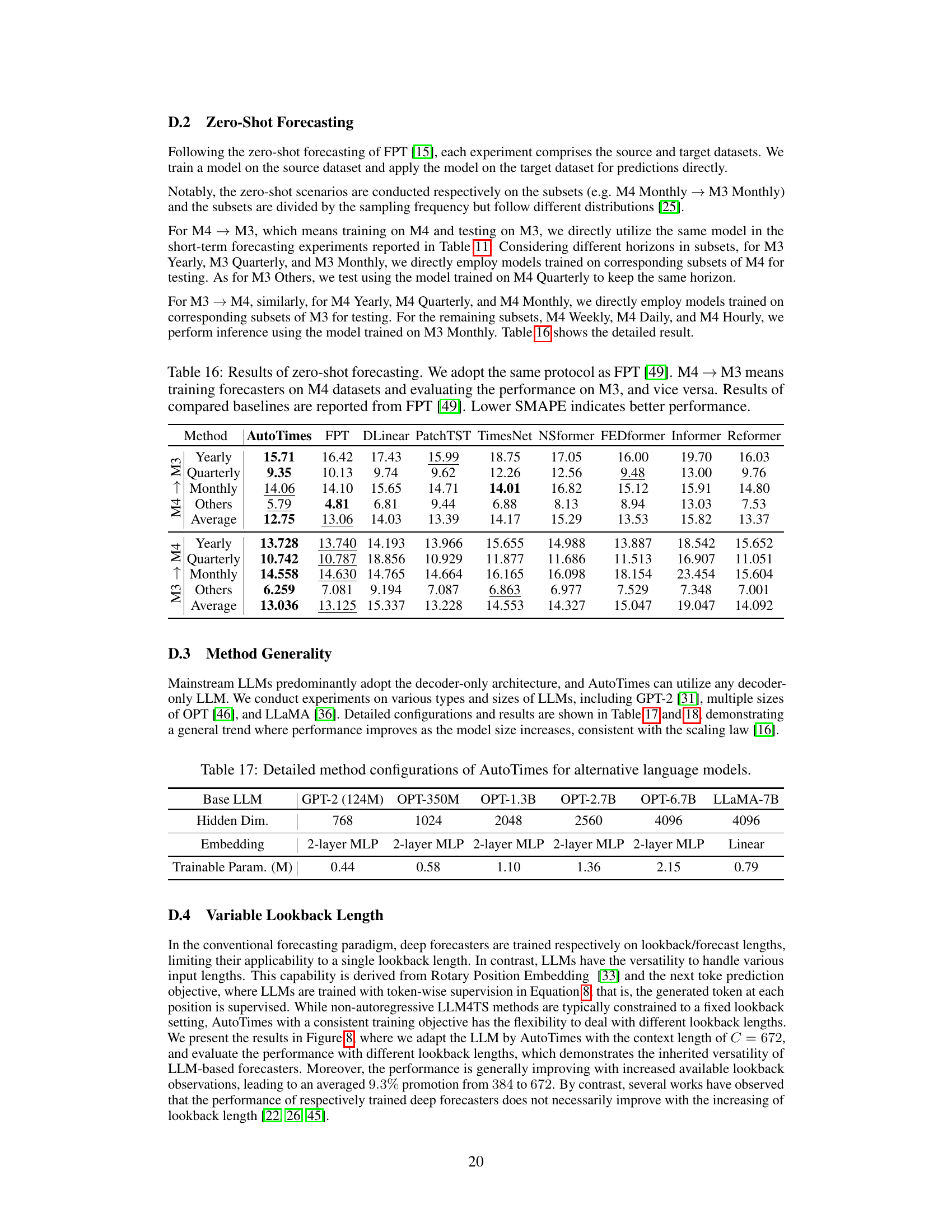
🔼 This table presents the results of zero-shot forecasting experiments. The models were trained on either the M4 or M3 dataset and then tested on the other dataset, to evaluate their ability to generalize to unseen data. The results are presented as the average Symmetric Mean Absolute Percentage Error (SMAPE), a common metric for evaluating time series forecasting accuracy. The table includes results for AutoTimes, and several baseline models (FPT, DLinear, PatchTST, TimesNet, NSFormer, FEDFormer, Informer, Reformer). Appendix D.2 provides more detailed results.
read the caption
Table 4: Zero-shot forecasting results in averaged SMAPE. M4 → M3 trains forecasters on the datasets of M4 and evaluates on M3, and vice versa. Detailed results are provided in Appendix D.2

🔼 This table presents the Mean Squared Error (MSE) and Mean Absolute Error (MAE) achieved by the AutoTimes model when using different large language models (LLMs) as the backbone. The LLMs tested include GPT-2 (124M), OPT-350M, OPT-1.3B, OPT-2.7B, OPT-6.7B, and LLaMA-7B. The results are averaged across several datasets and prediction horizons. The full results for each dataset and horizon can be found in Table 18.
read the caption
Table 5: Averaged results of alternative language models. Full results are provided in Table 18.

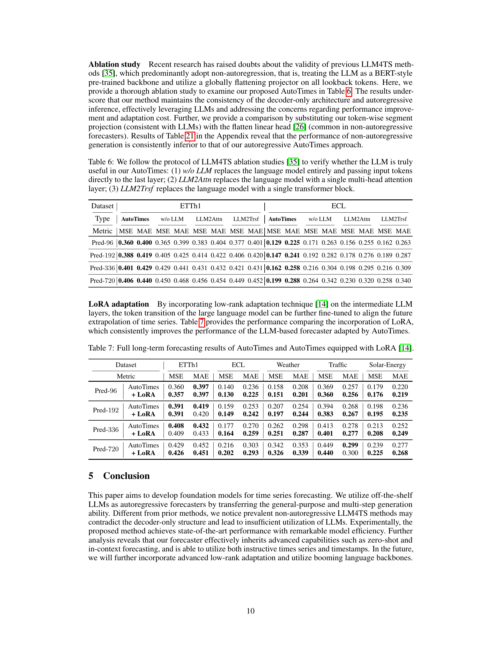
🔼 This table presents the ablation study results to verify the effectiveness of using LLMs in the AutoTimes model. Three variations of the model are compared against the baseline AutoTimes model: one without the LLM (w/o LLM), one using only a multi-head attention layer (LLM2Attn), and one using a single transformer block (LLM2Trsf). The results, measured by MSE and MAE, are shown for ETTh1 and ECL datasets for four different prediction horizons (Pred-96, Pred-192, Pred-336, Pred-720). This allows for a comparison of the performance impact of using different levels of the LLMs within the AutoTimes architecture.
read the caption
Table 6: We follow the protocol of LLM4TS ablation studies [35] to verify whether the LLM is truly useful in our AutoTimes: (1) w/o LLM replaces the language model entirely and passing input tokens directly to the last layer; (2) LLM2Attn replaces the language model with a single multi-head attention layer; (3) LLM2Trsf replaces the language model with a single transformer block.

🔼 This table presents the results of long-term time series forecasting experiments using a one-for-all approach, where a single model is trained on each dataset and used to make predictions for multiple forecast lengths (96, 192, 336, and 720). The AutoTimes model utilizes LLMs with a context length of 672, while other methods use an input length of 672 and an output length of 96. The table shows the average results across all forecast lengths, with complete results available in Table 10.
read the caption
Table 3: Long-term forecasting results of one-for-all: we conduct rolling forecasting with a single model trained on each dataset and accomplish four desired forecast lengths in {96, 192, 336, 720}. AutoTimes adapt LLMs with the context length C = 672. We set the input length L = 672 and output length F = 96 in other methods. All results are averaged. Full results is provided in Table 10.
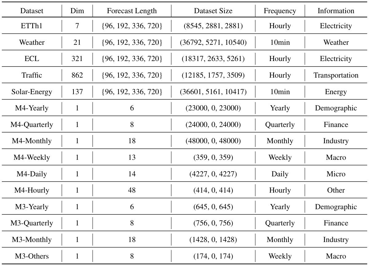
🔼 This table details the characteristics of the datasets used in the paper’s experiments. It lists the name of each dataset, the number of variables (Dim), the forecast lengths considered, the total number of data points in the training, validation, and testing sets, the sampling frequency (e.g., hourly, daily), and a brief description of the data’s information.
read the caption
Table 8: Detailed dataset descriptions. Dim denotes the variate number. Dataset Size denotes the total number of time points in (Train, Validation, Test) splits respectively. Forecast Length denotes the future time points to be predicted. Frequency denotes the sampling interval of time points.

🔼 This table presents the complete results of using different LLMs in the AutoTimes model. The context length is fixed at 672 for all experiments. The table shows the Mean Squared Error (MSE) and Mean Absolute Error (MAE) for different forecast horizons (96, 192, 336, and 720) across various datasets (ECL, ETTh1, Traffic, and Weather). The results allow for a comparison of model performance across different LLMs of varying sizes.
read the caption
Table 18: Full Results of alternative LLMs, which are adapted with the context length C = 672.

🔼 This table shows the performance of the AutoTimes model in terms of Mean Squared Error (MSE) and Mean Absolute Error (MAE) for four different forecasting horizons (96, 192, 336, and 720). The results are presented for four different datasets (ETTh1, ECL, Weather, and Traffic). For each dataset and horizon, the table provides the average MSE and MAE along with their standard deviations, calculated across three independent runs with different random seeds. This demonstrates the stability and robustness of AutoTimes.
read the caption
Table 9: Performance and standard deviations of AutoTimes. Results come from three random seeds.
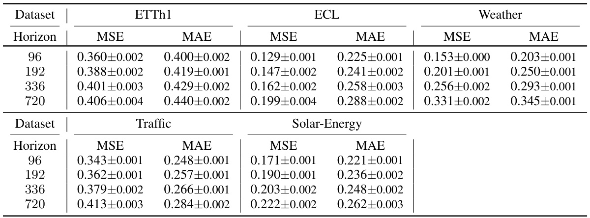
🔼 This table presents the mean and standard deviation of the MSE and MAE metrics for the AutoTimes model across different datasets (ETTh1, ECL, Weather, Traffic, Solar-Energy) and forecasting horizons (96, 192, 336, 720). The results are averaged across three different random seeds to show the model’s stability and reliability. Lower MSE and MAE values indicate better forecasting performance.
read the caption
Table 9: Performance and standard deviations of AutoTimes. Results come from three random seeds.
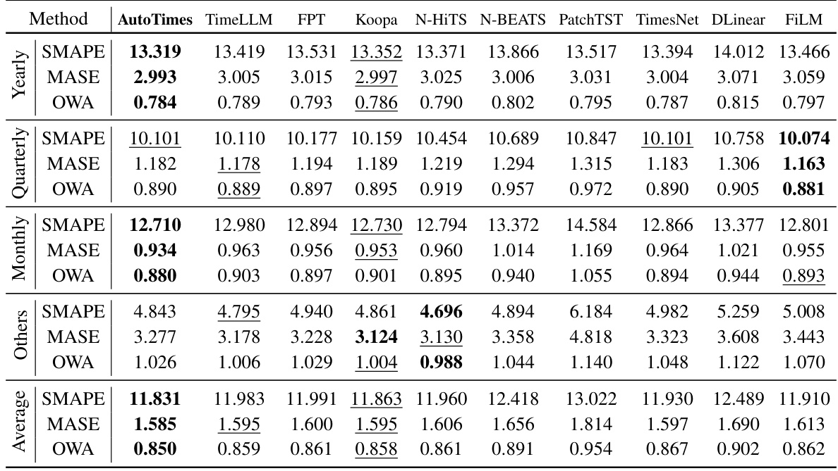
🔼 This table presents the average results of short-term time series forecasting on the M4 benchmark dataset. It compares the performance of AutoTimes against several state-of-the-art forecasting methods, including TimeLLM, FPT, Koopa, N-HiTS, DLinear, PatchTST, TimesNet, FiLM, and N-BEATS, across three evaluation metrics: SMAPE, MASE, and OWA. The full, detailed results for each method can be found in Table 11.
read the caption
Table 2: Average short-term forecasting results on the M4 [25]. Full results are provided in Table 11.

🔼 This table compares the results of several Large Language Model for Time Series (LLM4TS) methods reported in their original papers and the results reproduced by the authors of the current paper using the official code of those methods. The goal is to provide a reliable comparison of the performance of different methods on benchmark datasets.
read the caption
Table 13: Results of LLM4TS methods from the original paper and our reproduction by official code.
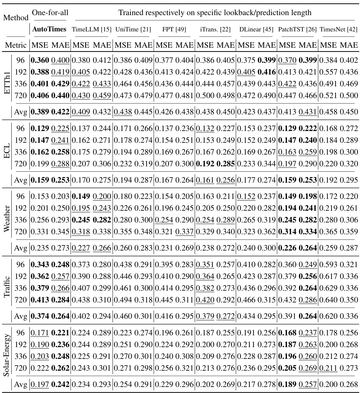
🔼 This table presents the results of long-term time series forecasting experiments using a one-for-all approach. A single model is trained on each dataset and then used to predict four different forecast lengths (96, 192, 336, and 720 time steps). AutoTimes uses a context length of 672, while other methods use an input length of 672 and an output length of 96. The table shows the average results across all four forecast lengths, with complete results available in Table 10. This setup tests the model’s ability to generalize to different prediction horizons without retraining.
read the caption
Table 3: Long-term forecasting results of one-for-all: we conduct rolling forecasting with a single model trained on each dataset and accomplish four desired forecast lengths in {96, 192, 336, 720}. AutoTimes adapt LLMs with the context length C = 672. We set the input length L = 672 and output length F = 96 in other methods. All results are averaged. Full results is provided in Table 10.

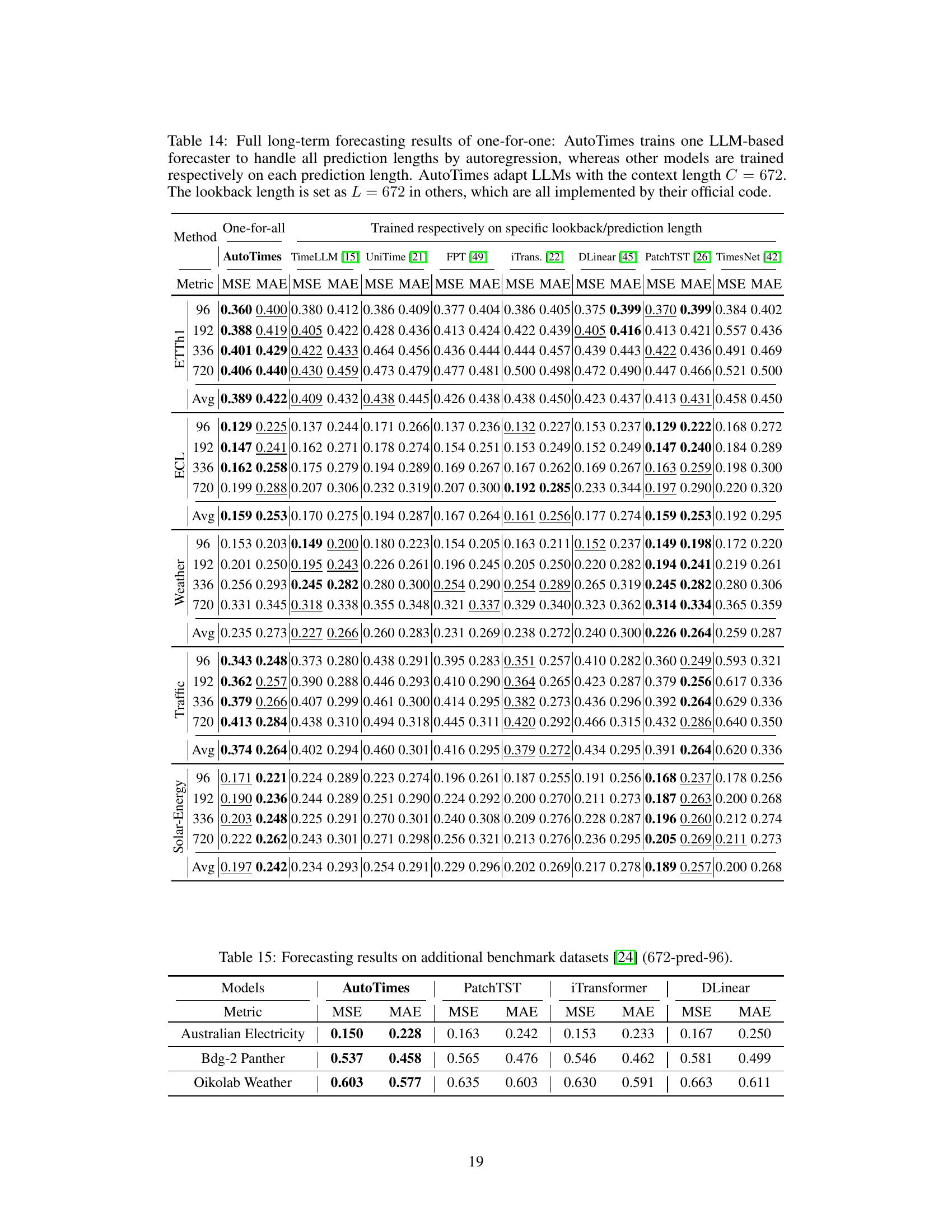
🔼 This table presents the results of forecasting experiments on three additional benchmark datasets, namely Australian Electricity, Bdg-2 Panther, and Oikolab Weather. The experiments use a lookback length of 672 time steps and predict the next 96 time steps. The table compares the performance of AutoTimes against three other state-of-the-art forecasting models: PatchTST, iTransformer, and DLinear. The metrics used for comparison are Mean Squared Error (MSE) and Mean Absolute Error (MAE).
read the caption
Table 15: Forecasting results on additional benchmark datasets [24] (672-pred-96).

🔼 This table presents the results of long-term forecasting experiments using a one-for-all approach. A single model is trained on each dataset and used to predict four different forecast lengths (96, 192, 336, and 720 time steps). AutoTimes uses a context length of 672, while other methods use an input length of 672 and an output length of 96. The table shows the average results across all forecast lengths, with full details available in Table 10.
read the caption
Table 3: Long-term forecasting results of one-for-all: we conduct rolling forecasting with a single model trained on each dataset and accomplish four desired forecast lengths in {96, 192, 336, 720}. AutoTimes adapt LLMs with the context length C = 672. We set the input length L = 672 and output length F = 96 in other methods. All results are averaged. Full results is provided in Table 10.

🔼 This table shows the different configurations used for AutoTimes when using different base LLMs. It lists the base large language model (LLM) used, the hidden dimension of the model’s layers, the type of embedding used (2-layer MLP or Linear), and the number of trainable parameters (in millions) for each configuration. The variations demonstrate the adaptability of AutoTimes to various LLMs.
read the caption
Table 17: Detailed method configurations of AutoTimes for alternative language models.
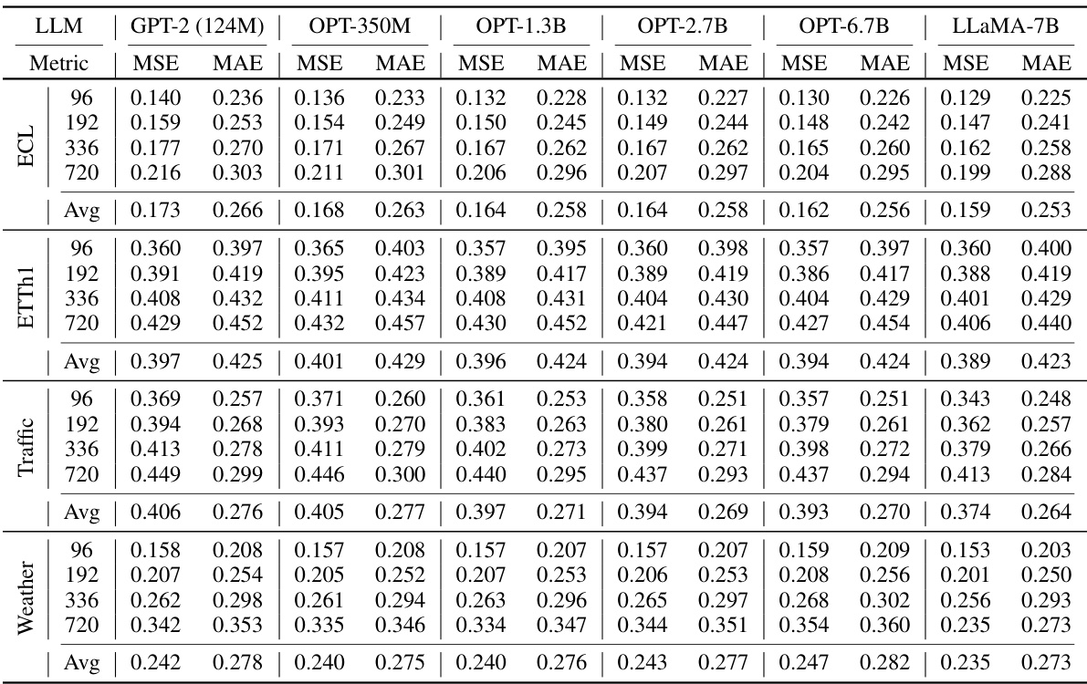
🔼 This table presents the results of experiments using different large language models (LLMs) for time series forecasting. The models tested include GPT-2 (124M), OPT-350M, OPT-1.3B, OPT-2.7B, OPT-6.7B, and LLaMA-7B. The metrics used to evaluate performance are Mean Squared Error (MSE) and Mean Absolute Error (MAE) for the 96, 192, 336, and 720 time steps ahead. The table shows average performance across these metrics and time steps. Full details are available in Table 18.
read the caption
Table 5: Averaged results of alternative language models. Full results are provided in Table 18.

🔼 This table presents the results of experiments using different strategies for selecting time series prompts in in-context forecasting. Four different strategies are compared: (P.1) using only the lookback window, (P.2) combining the lookback window with a prompt from the first 2F time points of the series, (P.3) combining the lookback window with a prompt from the last 2F time points of the series, and (P.4) combining the lookback window with a prompt from 2F time points of another series. The results are presented in terms of averaged error for four different time series frequencies (Yearly, Quarterly, Monthly, Others). Strategy P.2 and P.3 show improvement over P.1, while P.4 shows negative results as expected.
read the caption
Table 19: Effects of different strategies to retrieve time series as prompts for in-context forecasting.

🔼 This table presents the results of an ablation study on different prompt selection strategies for in-context forecasting. The study compares the performance of using different methods to select the time series prompts that are concatenated with the lookback window to form the context for prediction. The strategies include using the first 2F time points, the last 2F time points, randomly selected time points, and time points from other uncorrelated time series. The average error for each strategy is reported, illustrating the significant impact of prompt engineering on forecasting performance and highlighting the importance of using relevant and periodic time series prompts.
read the caption
Table 20: Strategies to select time series prompts based on periodicity for in-context forecasting.

🔼 This table presents the ablation study comparing the performance of AutoTimes with a variant called ‘FlattenHead’. FlattenHead replaces the segment-wise projection used in AutoTimes with a simpler flatten linear head, a common approach in non-autoregressive forecasting models. The results demonstrate that the performance of the non-autoregressive method (FlattenHead) is consistently inferior to the autoregressive approach (AutoTimes), highlighting the importance of AutoTimes’ autoregressive design for better performance.
read the caption
Table 21: Ablation study of the autoregression. FlattenHead replaces the segment-wise projection of AutoTimes by flatten and linear head [26], which is prevalent in non-autoregressive forecasters.
Full paper#
