↗ OpenReview ↗ NeurIPS Homepage ↗ Chat
TL;DR#
Training deep neural networks is challenging due to the complex, high-dimensional loss landscape. Understanding the curvature of this landscape is crucial for designing effective optimization algorithms. The Hessian matrix, while informative, is computationally expensive to calculate. The Gauss-Newton (GN) matrix offers a computationally cheaper approximation, but its properties in deep networks remain not fully understood.
This paper addresses this gap by providing a theoretical analysis of the GN matrix in deep neural networks. The authors derive tight bounds on the condition number of the GN matrix for deep linear networks and extend this analysis to two-layer ReLU networks, also examining the impact of residual connections. Their theoretical findings are validated empirically, providing valuable insights into how architectural design influences the conditioning of the GN matrix and consequently, the optimization process.
Key Takeaways#
Why does it matter?#
This paper is crucial for researchers in deep learning optimization because it provides theoretical insights into the Gauss-Newton matrix, a key component in many adaptive optimization methods. The tight bounds on the condition number offer a better understanding of training dynamics, enabling the design of improved architectures and optimization strategies. This work opens new avenues for research in understanding the influence of architectural choices on optimization landscape.
Visual Insights#

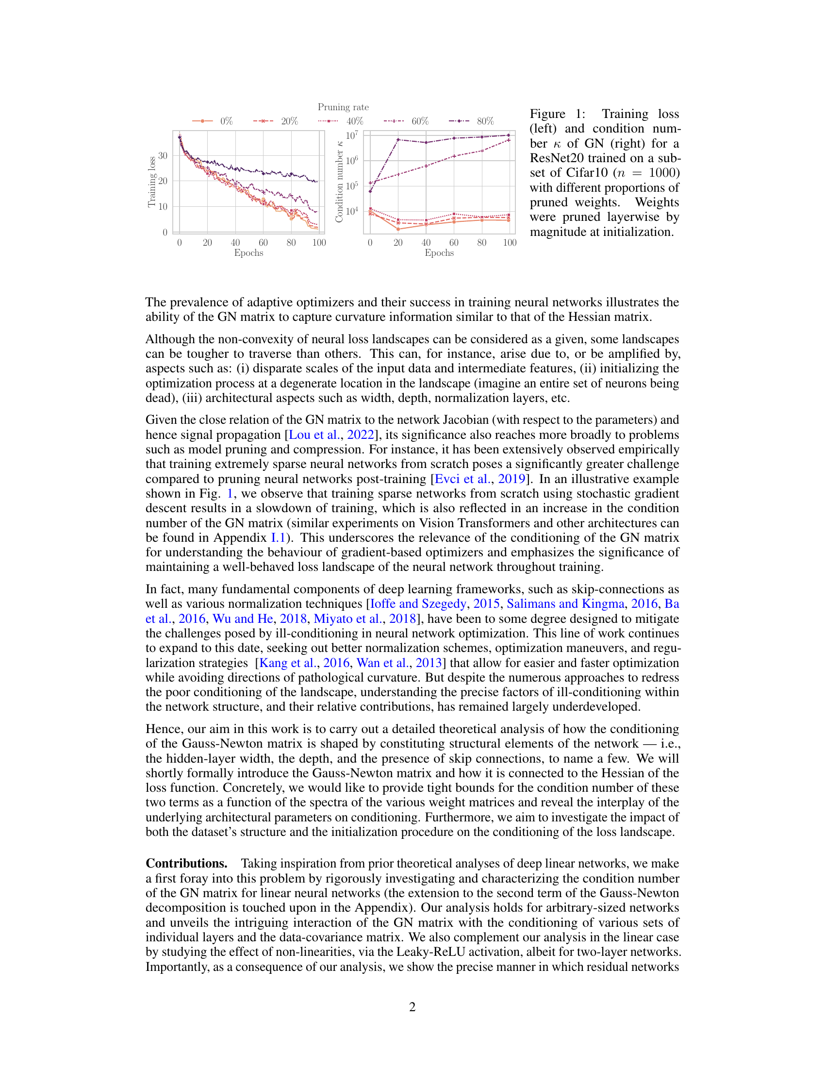
This figure shows the training loss and condition number of the Gauss-Newton (GN) matrix for a ResNet20 model trained on a subset of the CIFAR-10 dataset. Different lines represent different proportions of weights pruned from the network before training. The results indicate that pruning a larger proportion of weights leads to a higher condition number and slower convergence, as shown by the increased training loss. This highlights the relationship between weight pruning, GN matrix condition number and training performance.
In-depth insights#
GN Matrix Bounds#
The Gauss-Newton (GN) matrix is crucial for understanding neural network optimization, acting as a Hessian approximation. This paper focuses on deriving bounds for the GN matrix’s condition number, a key indicator of optimization difficulty. Tight bounds are established for deep linear networks of arbitrary depth and width, providing a theoretical understanding of how network architecture influences the conditioning of the optimization landscape. The analysis is extended to include non-linear (ReLU) networks and architectural components such as residual connections. Empirical validation confirms the theoretical bounds and highlights the impact of key architectural choices on GN matrix conditioning. This analysis offers valuable insights into designing well-conditioned neural networks, ultimately leading to more efficient and robust training.
Network Architectures#
The analysis of network architectures in deep learning is crucial for understanding and improving model performance. Depth significantly impacts the optimization landscape, often leading to challenges in training very deep networks. The authors explore the influence of depth on the Gauss-Newton matrix, demonstrating how it affects the conditioning and potentially slowing down convergence. Width, another critical architectural component, is also examined, showing how increasing the width of layers can positively influence conditioning, thus facilitating faster and more stable training. The study includes an investigation of residual connections, which are found to improve conditioning and enable the training of much deeper networks, highlighting their beneficial role in navigating complex loss landscapes. Non-linearities introduced by activation functions like ReLU also play a part, affecting the GN matrix’s condition number and influencing optimization dynamics. The impact of architectural choices such as the presence of skip connections or batch normalization are addressed, showcasing their potential to mitigate ill-conditioning and enhance overall training efficiency. Overall, the research provides theoretical insights and empirical evidence supporting the importance of considering these architectural factors for better training performance and optimization.
Non-linear Activations#
The section on “Non-linear Activations” would delve into the effects of introducing non-linearity into the network’s architecture. This is crucial because linear networks, while simpler to analyze, lack the representational power needed for complex real-world tasks. The authors would likely explore how non-linear activation functions (like ReLU, Leaky ReLU, sigmoid, etc.) impact the GN matrix’s conditioning and the optimization landscape. This would involve investigating how the non-linearity interacts with the network’s Jacobian and the Hessian approximation and its effect on eigenvalues and eigenvectors. Key questions addressed would likely involve how different activation functions affect the curvature of the loss landscape, which functions are more robust to ill-conditioning, and whether the established bounds on the linear network condition number still hold or need modification in the non-linear case. The analysis could potentially involve theoretical bounds, simulations with varying network architectures and activation functions, and comparisons to the linear case. Empirical results may demonstrate how non-linear activations influence training dynamics, convergence speed, and the overall generalization performance of the network. The discussion would also likely highlight the trade-offs between different activation functions: simplicity vs. expressiveness and the influence on the overall network’s behavior.
Residual Networks#
The paper analyzes the impact of residual connections on the conditioning of the Gauss-Newton (GN) matrix in neural networks. Residual connections, by adding skip connections that bypass certain layers, are shown to improve the conditioning of the GN matrix. This is a significant finding because well-conditioned GN matrices are crucial for efficient and stable optimization in deep learning. The analysis reveals that residual connections mitigate ill-conditioning by influencing the spectral properties of the GN matrix, leading to faster convergence and better generalization. The authors provide both theoretical bounds and empirical evidence supporting this claim, indicating that residual connections act as a form of regularization, making the optimization landscape easier to navigate. This work contributes to a deeper understanding of the geometric properties of deep neural networks and offers valuable insights for designing more efficient and robust training algorithms. Furthermore, this analysis helps explain the effectiveness of residual networks in training very deep architectures, where ill-conditioning is a major challenge. The study’s findings have broader implications for the design and optimization of deep learning models.
Future Research#
The paper’s “Future Research” section would ideally delve into extending the theoretical analysis to encompass more complex neural network architectures, such as transformers, and investigate the impact of various normalization techniques (batch normalization, layer normalization, etc.) on the GN matrix conditioning. A crucial area for future work is developing tighter bounds for the condition number that are less sensitive to eigenvalue distribution and account for training dynamics. Investigating the interplay between different activation functions and GN matrix conditioning is also critical, along with analyzing how various regularization methods influence conditioning. Finally, empirical studies on larger-scale datasets and more diverse network architectures would strengthen the theoretical findings and provide more practical insights. Exploring the connections between the GN matrix and other Hessian approximations, like K-FAC, would provide a richer understanding of the optimization landscape and aid in the development of more efficient optimization algorithms. The development of computationally efficient methods for computing the GN matrix and its condition number is vital to facilitating large-scale empirical studies.
More visual insights#
More on figures

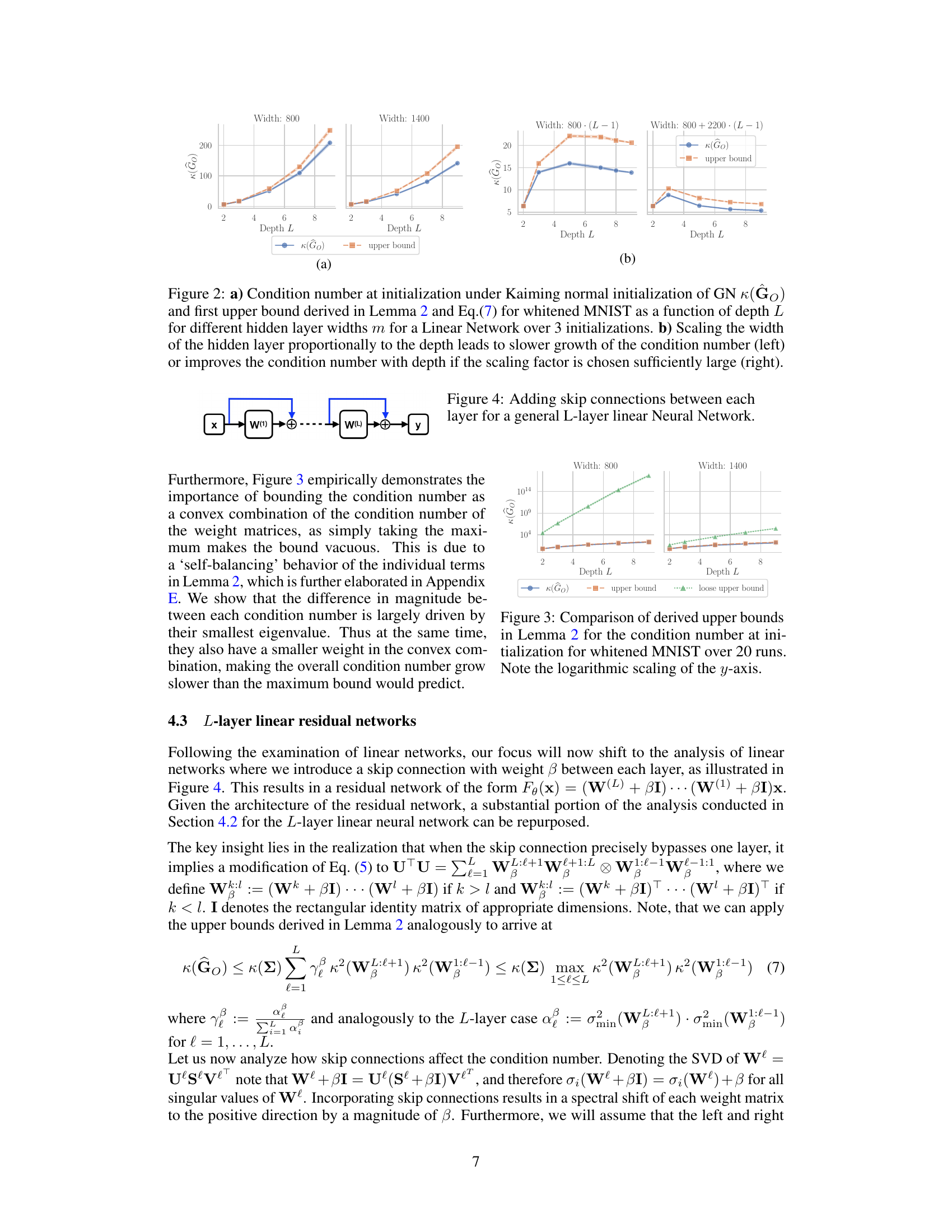
This figure shows the results of experiments on the effect of depth and width on the condition number of the Gauss-Newton matrix at initialization for a linear neural network. The left panel (a) shows the condition number and its upper bound for different network widths (m) and depths (L). The right panel (b) demonstrates the impact of scaling network width proportionally to depth, showing that appropriate scaling can mitigate the increase in condition number with depth.
This figure shows the results of experiments conducted to evaluate the condition number at initialization and the tightness of the upper bound derived in Lemma 2. Subfigure (a) displays the condition number κ(G₀) and its upper bound for different depths (L) and hidden layer widths (m) of a linear network, trained on the whitened MNIST dataset with Kaiming normal initialization. The results are averaged over three initializations. Subfigure (b) explores how scaling the width (m) proportionally with depth (L) affects the condition number. It shows that proportional scaling slows the growth, and sufficiently large scaling factors even improve the condition number with depth.

This figure shows the impact of network depth and width on the condition number of the Gauss-Newton (GN) matrix at initialization. Part (a) demonstrates the growth of the condition number with depth for fixed width, while part (b) illustrates how scaling the width proportionally to the depth mitigates this growth and can even lead to improvements in conditioning. The plots compare actual condition numbers to theoretical upper bounds derived in the paper.
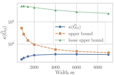
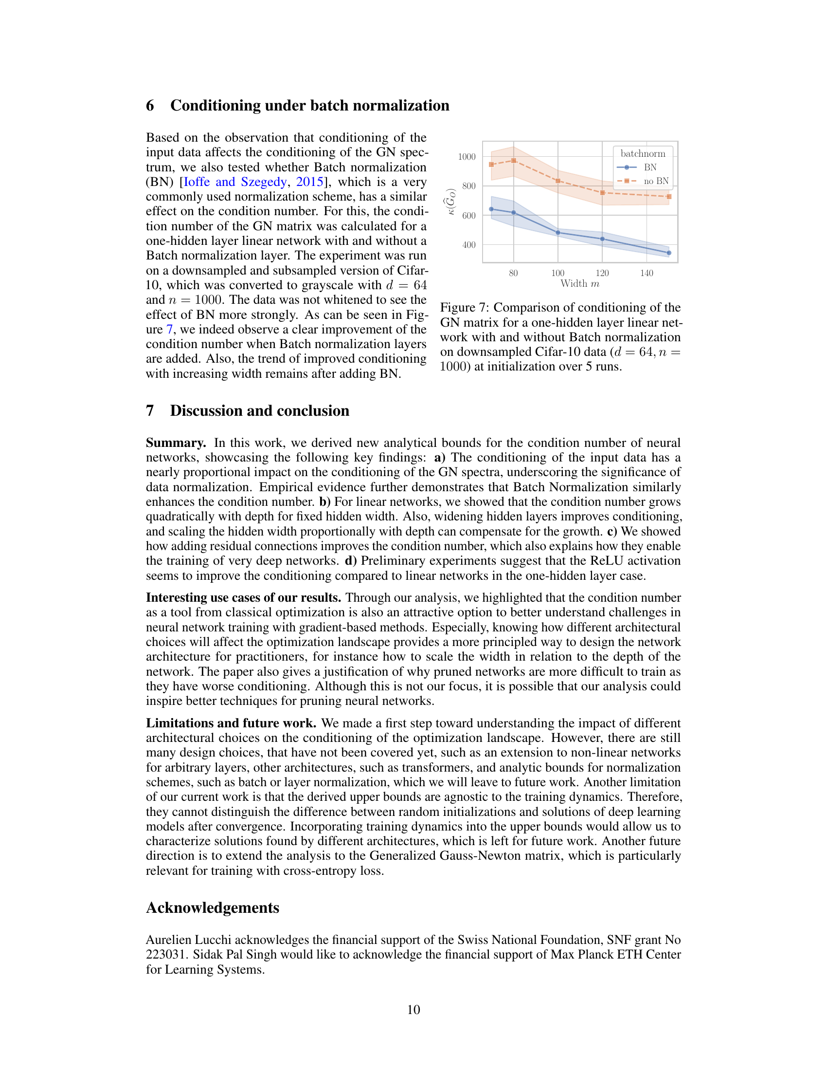
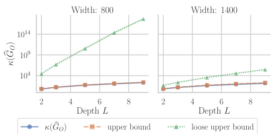
This figure compares the tightness of two upper bounds on the condition number of the Gauss-Newton matrix at initialization for a one-hidden layer neural network with linear activations. The ‘upper bound’ is derived using Weyl’s inequalities and a convex combination of the condition numbers of the weight matrices. The ’loose upper bound’ is a simpler bound that takes the maximum of the terms instead of the convex combination. The figure shows that the convex combination bound is much tighter than the loose bound. It also highlights the importance of this convex combination structure for obtaining a bound that is practically useful. The experiment is conducted on the whitened MNIST dataset, with a y-axis using a logarithmic scale.
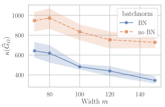
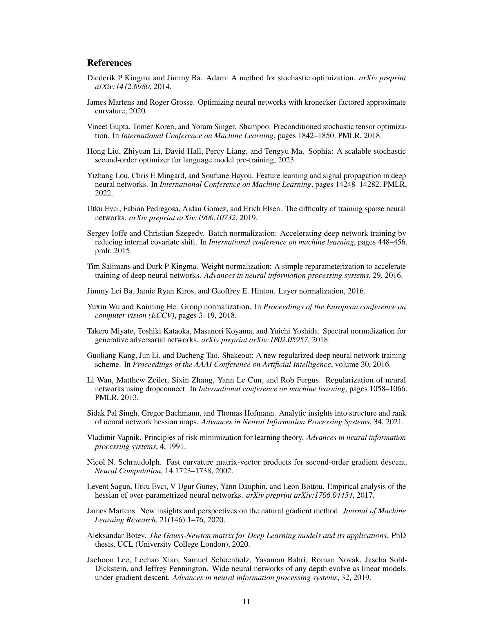
The figure compares the conditioning (condition number) of the Gauss-Newton (GN) matrix for a single-hidden-layer linear neural network with and without batch normalization. The experiment was conducted on a downsampled and subsampled grayscale version of the CIFAR-10 dataset (64 dimensions, 1000 samples). The plot shows the average condition number across five runs, with error bars indicating variability. The key observation is that adding batch normalization significantly improves the conditioning of the GN matrix, suggesting that batch normalization might help to mitigate the ill-conditioning effects frequently observed in neural network optimization. The trend of better conditioning with increasing width is maintained after including the batch normalization layer.

This figure shows the results of experiments conducted on a linear two-layer CNN. The experiments aimed to investigate the effect of kernel size and number of filters on the condition number of the Gauss-Newton matrix at initialization. The experiments were performed on a whitened subset of the MNIST dataset. The results indicate that increasing the number of filters leads to a higher condition number, analogous to increasing the depth in MLPs. Conversely, increasing the kernel size improves the conditioning, analogous to increasing the width in MLPs.

This figure shows the eigenvalue spectrum of the Gauss-Newton (GN) matrix at initialization and after 100 epochs of training. The left panel displays the ordered eigenvalues, highlighting the smallest non-zero eigenvalue (marked with a star). The right panel demonstrates the sensitivity of the condition number to variations in the estimated matrix rank, showcasing how small changes in the rank significantly impact the condition number, especially after 100 epochs.

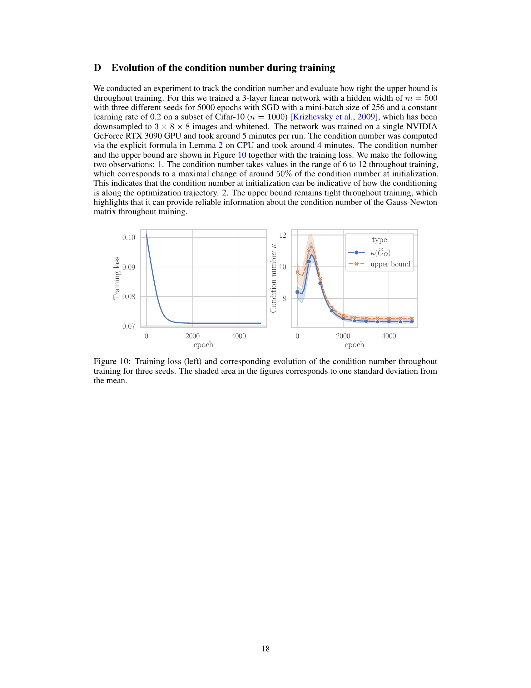
This figure shows the training loss and the condition number of the Gauss-Newton matrix throughout the training process for three different random initializations of a three-layer linear network with a hidden layer width of 500. The experiment uses SGD with a constant learning rate of 0.2 trained on a subset of Cifar-10 (1000 images) that have been downsampled and whitened. The plot highlights two key observations: 1. The condition number remains relatively stable (6-12) across the training process, indicating its value at initialization may be predictive of its behavior during optimization. 2. The upper bound on the condition number, derived from theoretical analysis in the paper, remains tight throughout training, confirming the accuracy of the theoretical result.
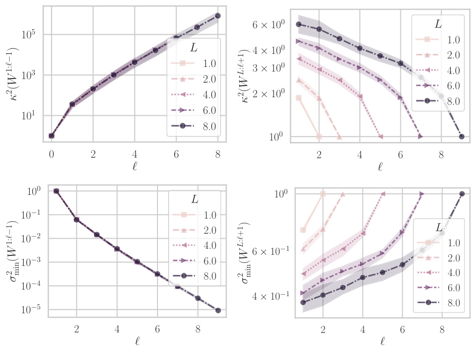
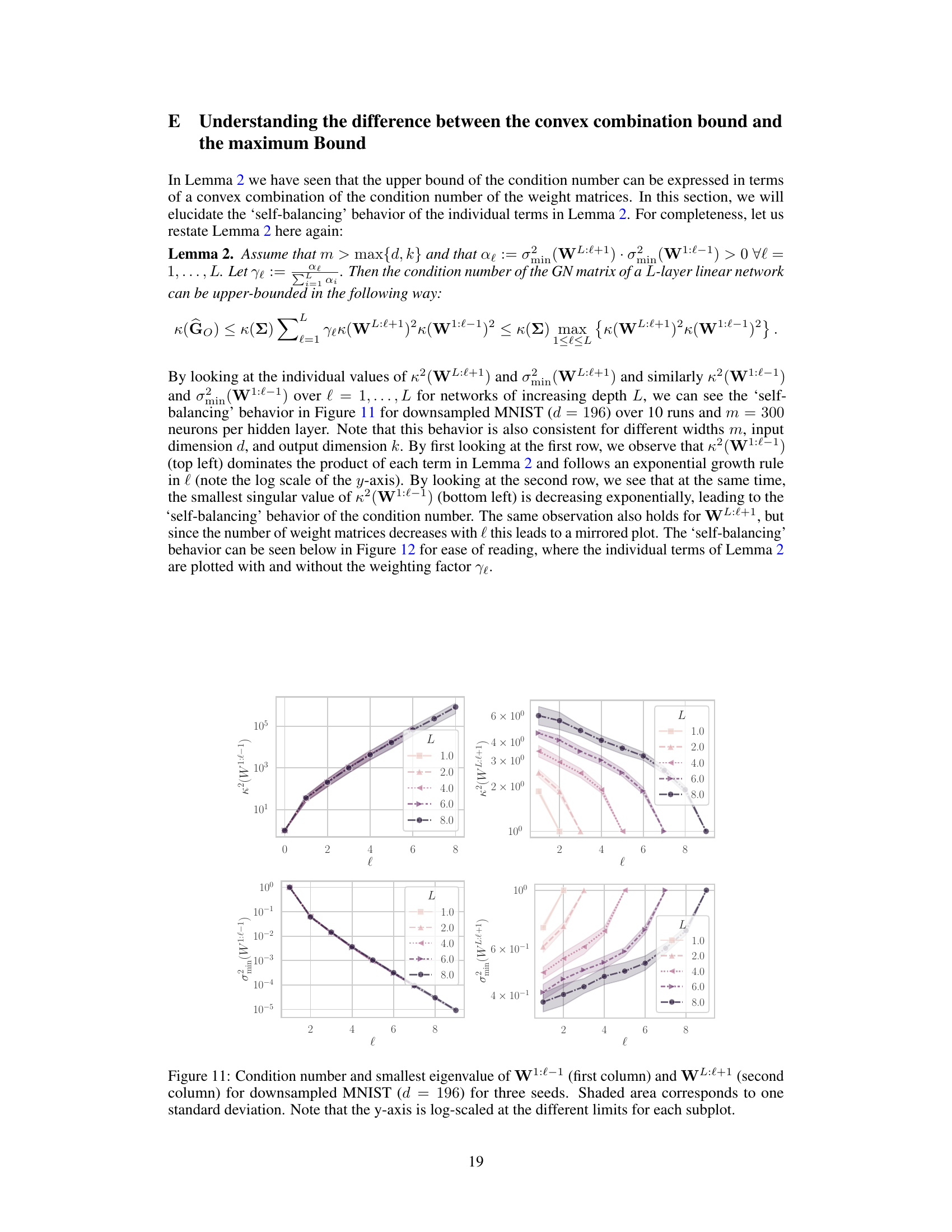
This figure shows the behavior of the condition number and the smallest eigenvalue of the weight matrices W1:l−1 and WL:l+1 for different depths (L) of a linear neural network. The data used is a downsampled version of the MNIST dataset. The plots illustrate how the condition number (a measure of how ill-conditioned the matrix is) and the smallest singular value change as the number of layers (l) increases. The shaded regions represent one standard deviation across three different random initializations of the network weights.
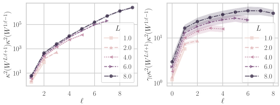
This figure shows the results of experiments on the condition number of the Gauss-Newton matrix at initialization for linear networks. The left plot (a) shows the condition number and an upper bound as a function of depth for different hidden layer widths. The right plot (b) demonstrates the effect of scaling the width of the hidden layer proportionally to the depth, showing that this approach can lead to either slower growth or improved conditioning of the condition number.

This figure shows the training loss and the condition number of the Gauss-Newton (GN) matrix for a ResNet20 model trained on a subset of the CIFAR-10 dataset. Different proportions of the model’s weights were pruned (removed) before training, and the impact of this pruning on both the training loss and the GN matrix’s condition number is visualized. The condition number of the GN matrix is a measure of its conditioning—how well-behaved the optimization landscape is around the current weights. A higher condition number indicates a more ill-conditioned problem, implying difficulties in training. As shown in the plots, pruning a greater proportion of weights prior to training results in a higher training loss and a larger GN matrix condition number, indicating more challenges during the training process.

This figure shows the training loss and condition number of the Gauss-Newton (GN) matrix for a ResNet20 model trained on a subset of the CIFAR-10 dataset. Different proportions of weights were pruned layerwise by magnitude at initialization. The left plot displays the training loss curves for different pruning rates (0%, 20%, 40%, 60%, 80%), while the right plot shows the corresponding condition number of the GN matrix. The figure illustrates the relationship between weight pruning, training loss, and the GN matrix’s condition number. Higher condition numbers generally suggest a more difficult optimization landscape.

This figure shows the training loss and condition number of the Gauss-Newton (GN) matrix for a ResNet20 model trained on a subset of the CIFAR-10 dataset. Different lines represent different proportions of weights that were pruned before training. The pruning was performed layerwise, based on the magnitude of the weights at initialization. The figure illustrates the relationship between weight pruning, training progress, and the conditioning of the GN matrix, highlighting how pruning can impact optimization.
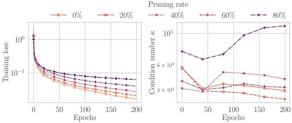
This figure shows the training loss and condition number of the Gauss-Newton (GN) matrix for a ResNet20 model trained on a subset of the CIFAR-10 dataset. Different proportions of weights were pruned layerwise by magnitude at initialization. The left plot displays the training loss curves for different pruning rates (0%, 20%, 40%, 60%, 80%), revealing how pruning affects training progress. The right plot illustrates the corresponding condition numbers of the GN matrix for each pruning rate, indicating the impact of pruning on the optimization landscape’s conditioning. The experiment demonstrates how increased pruning negatively impacts training and increases the condition number, which could explain why training sparse networks from scratch is more challenging.

This figure shows the training loss and condition number for different widths (15, 20, 50, 100, 150, 200) of a one-hidden layer feed-forward network trained on a subset of MNIST (1000 samples). The network is trained using SGD with a fixed learning rate, chosen via grid search. The plot demonstrates that increasing the width of the hidden layer improves both the convergence speed (training loss decreases faster) and the conditioning of the network (condition number is lower and more stable during training).

This figure compares the condition number of the Gauss-Newton (GN) matrix for a linear neural network with a hidden width of 3100, trained on the CIFAR-10 dataset, both with and without data whitening. The y-axis is logarithmic, showing a substantial difference in the condition number between the whitened and un-whitened data, particularly as the network depth increases. Data whitening significantly improves the conditioning, which is crucial for efficient training.
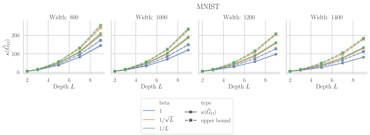
This figure presents the results of experiments on the condition number at initialization for linear networks. The left panel (a) shows that the condition number increases as the network depth increases. The right panel (b) shows that if the width of the hidden layers is scaled proportionally with the depth, the growth of the condition number slows down or even improves with increasing depth. This supports the main finding of the paper that the condition number of the Gauss-Newton matrix is affected by the width and depth of the network.

This figure shows the results of experiments on the condition number at initialization for linear networks with different depths and widths. The left part (a) shows the condition number and its upper bound for different widths, while the right part (b) illustrates how scaling the width proportionally to the depth affects the condition number.
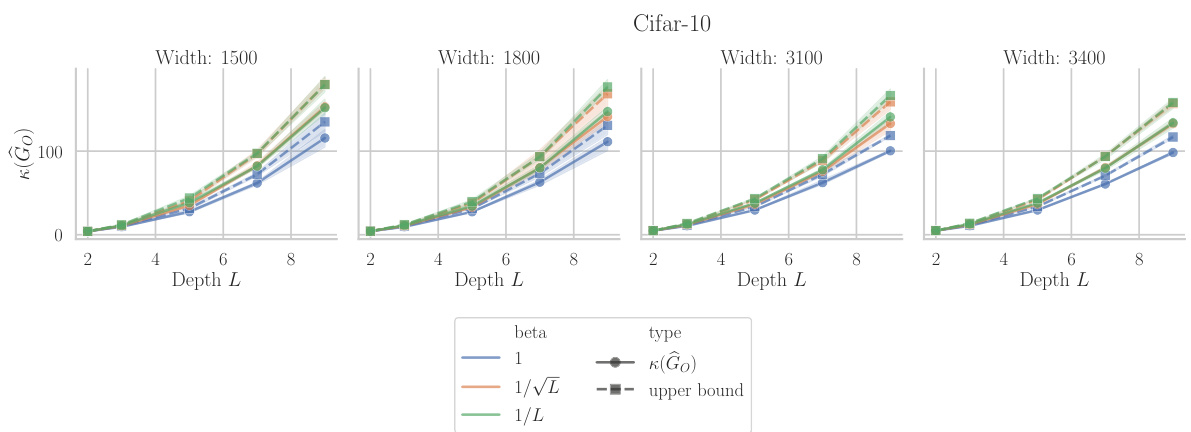
Figure 2 presents the results of an experiment conducted to analyze how the condition number of the Gauss-Newton (GN) matrix changes with the depth and width of the network. The left subplot (a) shows that the condition number at initialization increases with depth for different hidden layer widths (m) and compares it to the upper bound derived in Lemma 2 and Equation 7. The right subplot (b) demonstrates that scaling the hidden layer width proportionally to the depth can either slow down or improve the condition number depending on the proportionality factor.

This figure shows the impact of network depth and width on the condition number of the Gauss-Newton (GN) matrix at initialization for a linear neural network. Subfigure (a) plots the condition number against depth for different widths, showing a quadratic increase with depth for fixed width and a slower growth when width scales proportionally with depth. Subfigure (b) further illustrates that appropriately scaling width with depth can even improve conditioning as depth increases.
Full paper#
