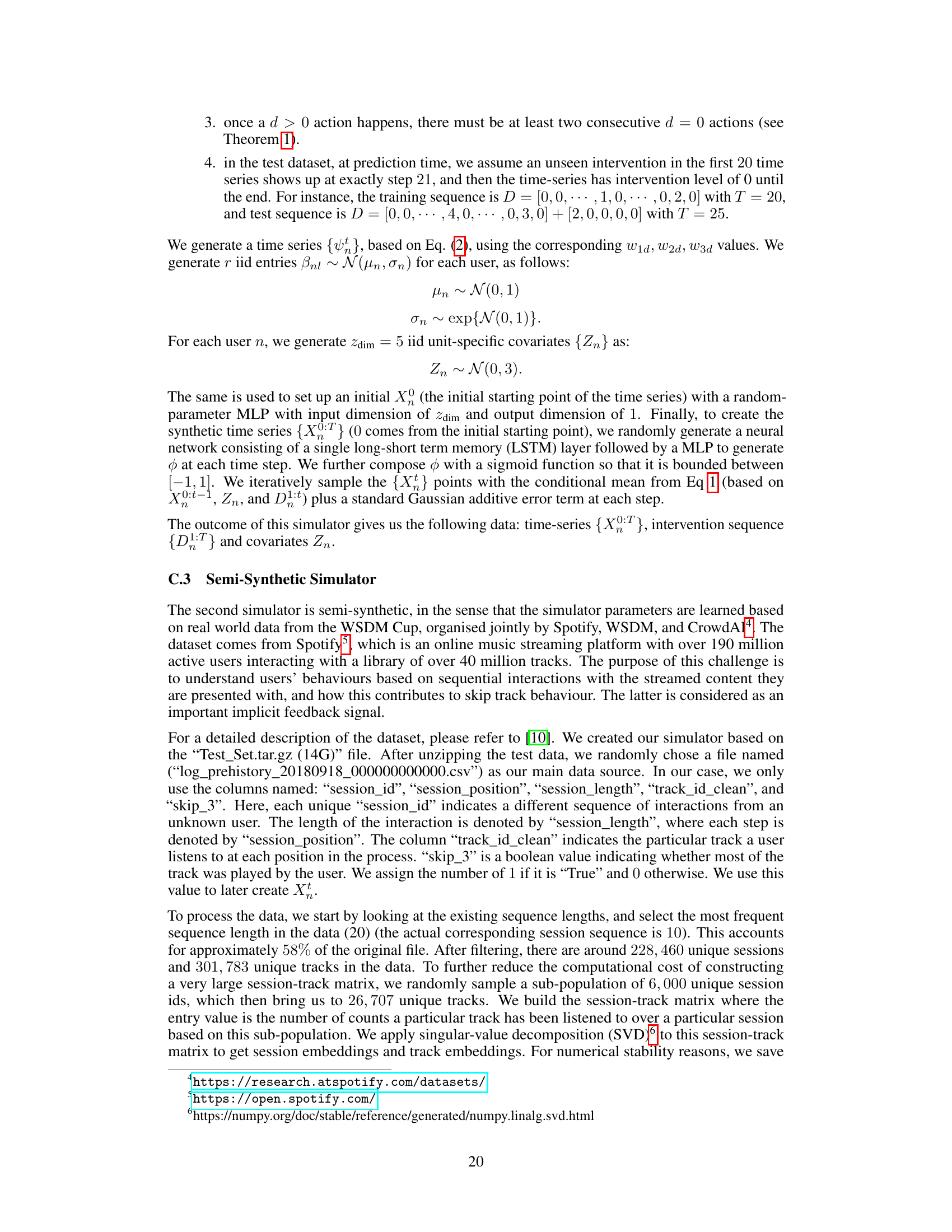
TL;DR#
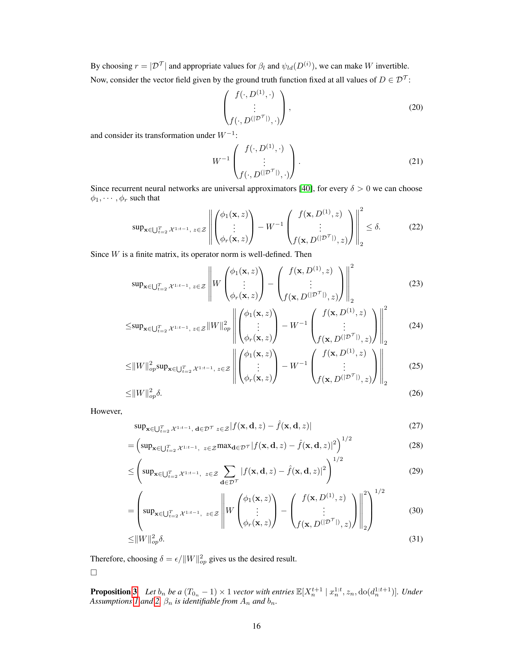
Many real-world problems involve predicting outcomes of sequential interventions (e.g., drug treatments, marketing campaigns). Standard methods struggle when interventions are complex and data is sparse, making it hard to generalize predictions. This is problematic as these methods often rely on poorly understood assumptions.
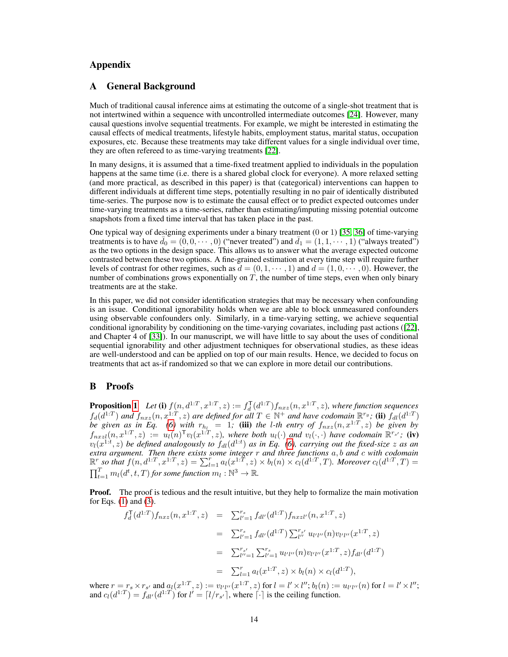
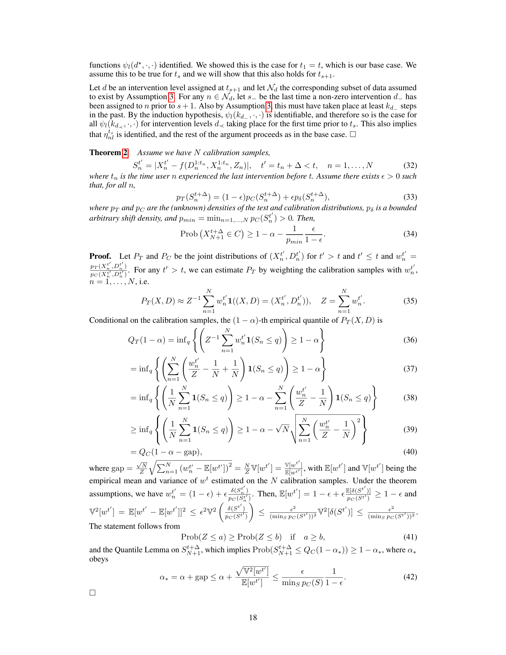
This paper proposes a structured approach, CSI-VAE, explicitly modeling the composition of interventions over time. CSI-VAE offers better predictive performance compared to black-box models, particularly in sparse data scenarios, by leveraging the structure of the interventions. It also offers identifiability guarantees under certain conditions, ensuring that predictions are reliable and generalizable. The method combines the flexibility of a variational autoencoder with an explicit model of compositionality.
Key Takeaways#
Why does it matter?#
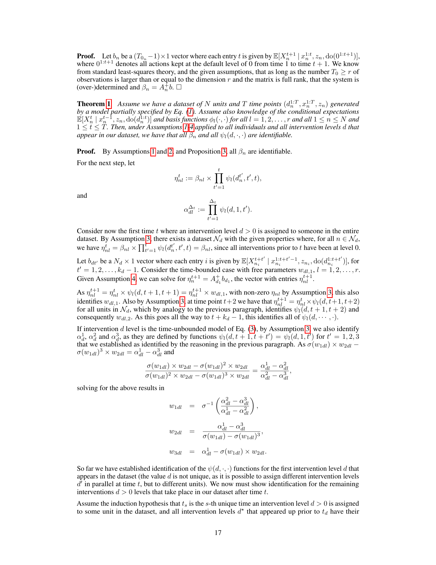
This paper is important because it presents a novel approach to predict the effects of sequential interventions, particularly in scenarios with sparse data and high-dimensional action spaces. It offers identifiability guarantees under specific conditions, which is crucial in causal inference. The developed CSI-VAE model combines compositional modeling with a variational autoencoder, offering advantages over traditional black-box methods. This work opens avenues for further investigation into structured causal representation learning and reliable prediction in complex intervention settings, relevant to various fields dealing with sequential decision-making and causal effect estimation.
Visual Insights#
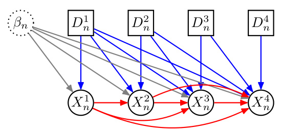
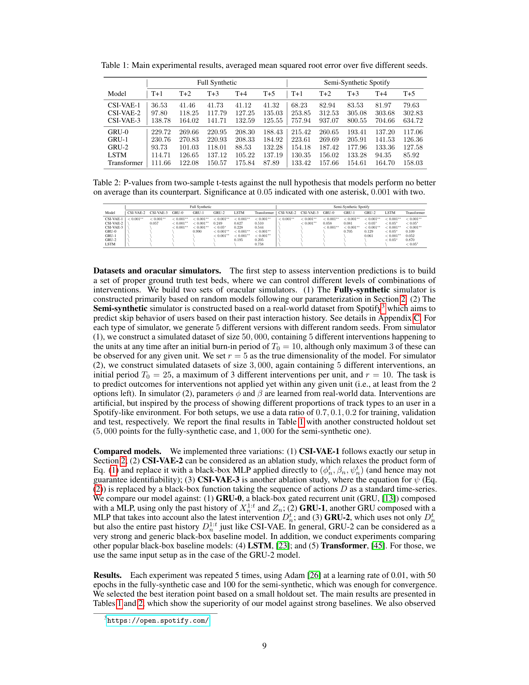
🔼 This figure shows a graphical model representing the causal relationships between actions (interventions), latent variables, and observed outcomes within a single unit (n). The actions (D1, D2, D3, D4) are shown as square nodes, and the observed outcomes (X1, X2, X3, X4) are depicted as circular nodes. A latent random effect (βn) influences both the actions and the outcomes, represented by the gray arrows. The blue arrows indicate the direct effect of each action on subsequent outcomes, highlighting the sequential nature of the interventions. Red curved arrows represent potential temporal dependencies between outcomes. The figure emphasizes the complexity of modeling the combined effects of sequential interventions due to the intricate interplay of actions, latent factors, and temporal dynamics.
read the caption
Figure 1: Within unit n, actions Dhe interact with (latent) random effect parameters ßn to produce behavior Xt represented as a dense graphical model with square vertices denoting interventions do(dhit) [33, 16]. Further assumptions will be required for the identifiability of the impact of in- terventions and their combination, including how temporal impact takes shape and the number of independent units of observation.

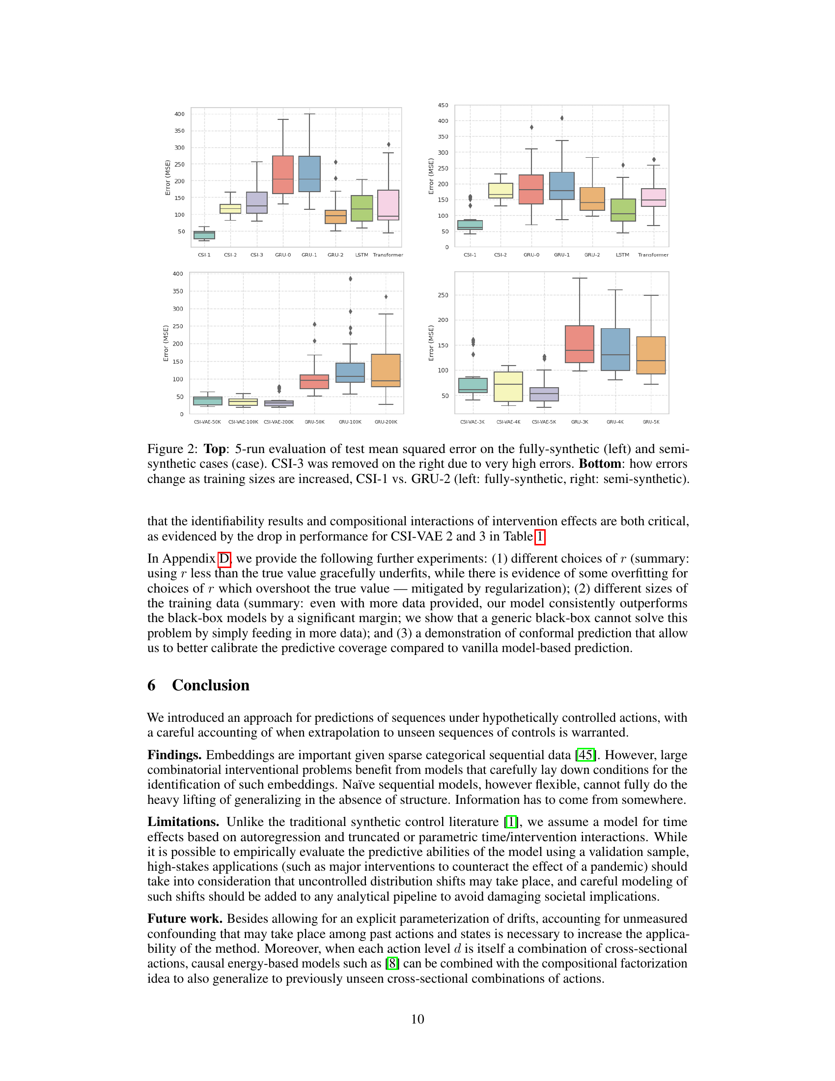
🔼 This table presents the main experimental results of the paper, comparing the performance of various models in predicting future behavioral sequences. The results are given as the average mean squared root error (MSE) across five different random seeds. The models are evaluated on two different datasets: a fully synthetic dataset and a semi-synthetic Spotify dataset. The table shows the MSE for each model at various time steps (T+1 to T+5), allowing for a comparison of model performance over time. The results are crucial for demonstrating the superiority of the proposed CSI-VAE models.
read the caption
Table 1: Main experimental results, averaged mean squared root error over five different seeds.
In-depth insights#
Compositional Effects#
The concept of “Compositional Effects” in sequential intervention studies centers on understanding how the impact of multiple interventions combines over time. A crucial aspect is disentangling individual intervention effects and determining how they interact to produce an overall outcome. Standard black-box models struggle with this because they lack the explicit representation of the compositional structure. The challenge lies in generalizing to novel intervention sequences not seen during training, especially under sparse data conditions where few combinations of interventions are observed. Therefore, methods explicitly modeling compositionality, such as those inspired by causal matrix factorization, are needed. These methods aim to isolate individual intervention effects into modules, revealing which data conditions enable the identification of combined effects across units and time points. Structure aids prediction by enabling the transfer and recombination of information learned from previously observed interventions. This contrasts with flexible yet generic black-box models, highlighting the advantages of incorporating structural assumptions for prediction in sparse, complex settings.
CSI-VAE Model#
The CSI-VAE model, a novel approach for predicting sequential interventions, cleverly combines the strengths of causal inference and deep learning. It addresses the challenge of generalizing to unseen intervention sequences, a common issue in sparse data settings, by explicitly modeling the compositional nature of sequential effects. The model elegantly leverages a structural approach inspired by causal matrix factorization, allowing for the isolation and recombination of intervention effects across time and units. This decomposition enhances generalization compared to traditional black-box models. The use of variational autoencoders (VAE) introduces flexibility and scalability, allowing for the handling of high-dimensional and sparse data. The model demonstrates improved predictive performance in sparse data scenarios, showcasing its ability to learn and extrapolate from limited information. CSI-VAE is further enhanced by robust uncertainty quantification techniques, promoting reliability and trustworthiness of predictions. In essence, it provides a powerful and practical framework for tackling complex sequential intervention settings within the realm of causal inference.
Identifiability#
The concept of identifiability in causal inference, particularly within the context of sequential interventions, is crucial for establishing the reliability and validity of causal effect estimations. Identifiability ensures that the causal effects of interest can be uniquely determined from the observed data, without ambiguity or confounding factors. In the realm of sequential interventions, identifiability becomes particularly challenging due to the complex interplay of multiple interventions over time. The presence of confounding variables, temporal dependencies between interventions, and sparse data conditions can significantly hinder the identification of causal effects. Therefore, careful consideration of the data generating mechanisms and underlying structural assumptions is necessary. The paper explicitly addresses these challenges by proposing a compositional model that breaks down the overall effects into simpler, identifiable modules. By specifying assumptions on how these modules interact, and the conditions under which the data is generated, the authors aim to guarantee identifiability, even in the presence of complex temporal patterns and scarce data points. This approach significantly contributes to advancing our understanding and capabilities in causal inference for dynamic systems.
Uncertainty Quantification#
The section on Uncertainty Quantification is crucial for evaluating the reliability of the model’s predictions, especially in high-stakes applications where the consequences of inaccurate predictions can be significant. The authors employ two main approaches: model-based and distribution-free methods. The model-based approach leverages the estimated parameters and error variance from the learned model to generate prediction intervals. However, this method’s simplicity comes at the cost of potentially underestimating uncertainty, failing to capture estimation error and data variability. The authors address this shortcoming by adopting a distribution-free approach, specifically, conformal prediction, which provides guaranteed coverage probabilities for prediction intervals regardless of the true data distribution. This robust method, while requiring a calibration dataset, offers a more reliable assessment of uncertainty and increased trust in the model’s predictions in complex real-world scenarios. Comparing the results from both approaches reveals valuable insights into the strengths and weaknesses of each method, highlighting the trade-off between simplicity and rigorous uncertainty quantification. The combination of these methods provides a more complete and nuanced understanding of the model’s predictive uncertainty.
Future Work#
The paper’s “Future Work” section suggests several promising avenues. Addressing unmeasured confounding is crucial for enhancing the model’s robustness in real-world scenarios where hidden factors influence outcomes. The authors also propose extending the model to handle combinations of cross-sectional actions, a significant advancement for capturing complex interventions. This would require incorporating causal energy-based models to improve generalization. Another key area is improving the handling of time-varying effects, potentially using parameter drift models to better capture temporal changes in treatment impact. Finally, they recognize the need for more sophisticated methods to handle high-dimensional discrete covariate spaces, suggesting research into novel dimensionality reduction techniques combined with advanced causal inference methods is merited.
More visual insights#
More on figures

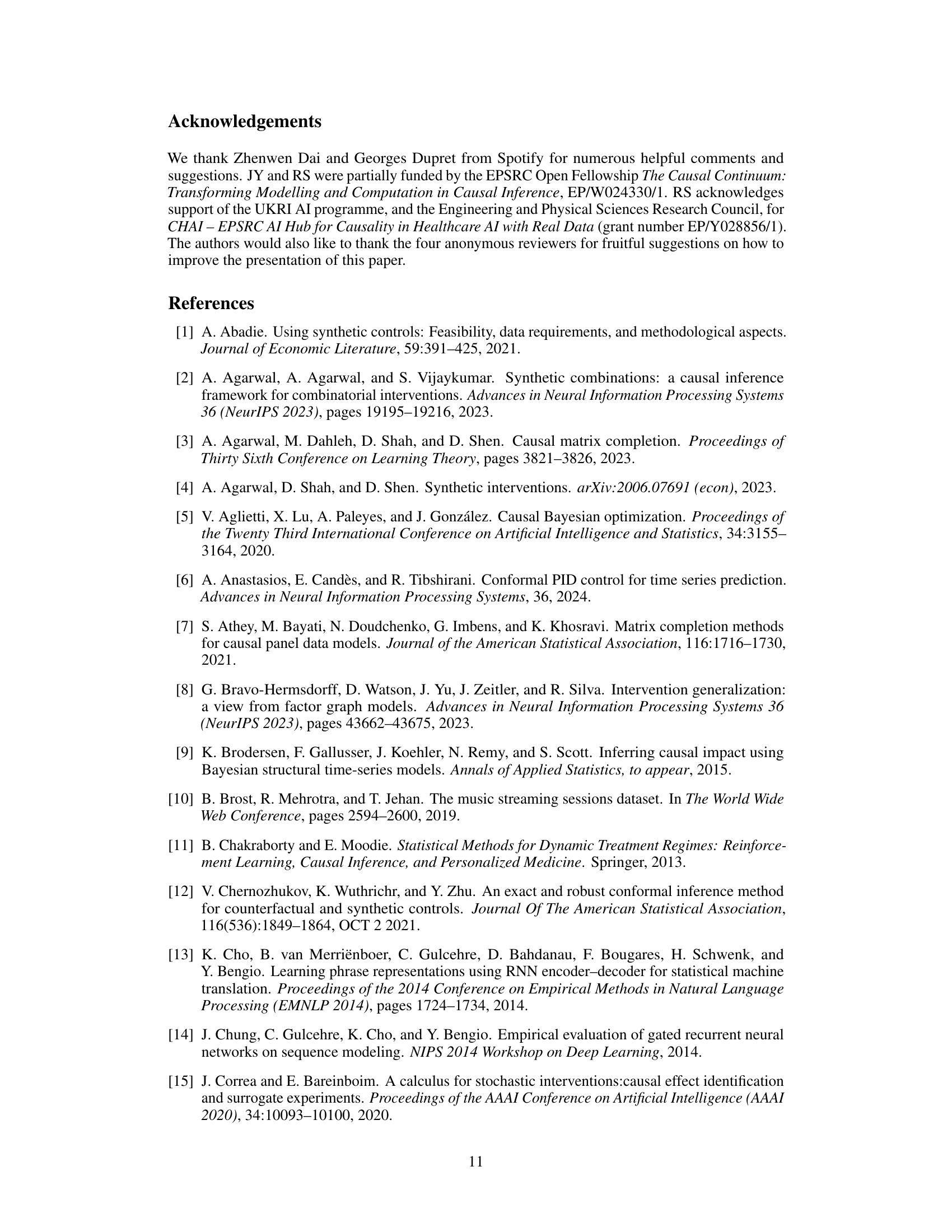
🔼 The figure displays box plots to compare the performance of CSI-VAE and GRU across different datasets. The top row presents the test mean squared error (MSE) for five different model setups in fully synthetic and semi-synthetic datasets. The bottom row shows how the MSE changes as the training dataset sizes increase for CSI-VAE-1 and GRU-2, again across the fully synthetic and semi-synthetic datasets. Note that CSI-VAE-3 is excluded from the right plot due to significantly higher errors compared to other models.
read the caption
Figure 2: Top: 5-run evaluation of test mean squared error on the fully-synthetic (left) and semi-synthetic cases (case). CSI-3 was removed on the right due to very high errors. Bottom: how errors change as training sizes are increased, CSI-1 vs. GRU-2 (left: fully-synthetic, right: semi-synthetic).

🔼 This boxplot shows the effect of varying the dimensionality parameter ‘r’ on the mean squared error (MSE) of the fully-synthetic dataset. The ground truth value of r is 5. The boxplot shows that using a smaller r (r=3) leads to underfitting (higher MSE), whereas using a larger r (r=10) can lead to overfitting (high variance) but can achieve lower MSE, indicating that the model benefits from a higher dimensional representation. Regularization techniques (L1 and L2 norms) are also shown to help mitigate the overfitting effect seen when r=10.
read the caption
Figure 3: Effect of changing r for the fully-synthetic dataset.

🔼 This figure shows six plots, each visualizing the reconstruction of a time series from the training data for the CSI-VAE-1 model. Each plot displays the real time series values (blue line) and the best reconstruction (orange line) for a specific user, along with the time steps on the x-axis. This figure helps illustrate the model’s ability to learn and reproduce complex patterns in the data. The visual comparison of the real and reconstructed time series provides a qualitative assessment of the model’s performance.
read the caption
Figure 4: Examples of reconstruction of training data for CSI-VAE-1 model.

🔼 This figure displays examples of reconstruction of training data using the CSI-VAE-1 model. It showcases how well the model reconstructs the original time series data for six different users. The plots compare the actual time series data (Real) against the model’s best reconstruction (Recon (best)), showing a close match between the two. Additionally, 95% confidence intervals are provided to give a sense of the uncertainty associated with the reconstruction.
read the caption
Figure 4: Examples of reconstruction of training data for CSI-VAE-1 model.

🔼 This figure demonstrates the prediction results of the CSI-VAE-1 model on synthetic data. It shows the actual time series of X for six different users (User 1 to User 6), along with their corresponding control paths and predictive paths. The control paths represent the expected behavior under no intervention, while the predictive paths are generated by the model. The vertical dashed lines indicate the timesteps where interventions occurred. The figure visually compares the model’s predictions (in green) against the actual observed values (in blue), and shows how well the model captures the effect of interventions on the system dynamics. The variation of each line represents the uncertainty of the model’s predictions.
read the caption
Figure 6: Demonstration of prediction, in the synthetic data case, for CSI-VAE-1.

🔼 This figure displays histograms of prediction errors at different time steps (T+1 to T+5) for the CSI-VAE-1 model. The histograms show the distribution of the differences between the model’s predictions and the true values of the target variable. The long tails indicate that the model occasionally makes large errors, although most predictions are relatively accurate. This is a common characteristic of many machine learning models, particularly for time series, where complex dependencies can make precise prediction challenging.
read the caption
Figure 7: Residual distribution examples for CSI-VAE-1. In general, we observe a very long tail effect across model predictions.
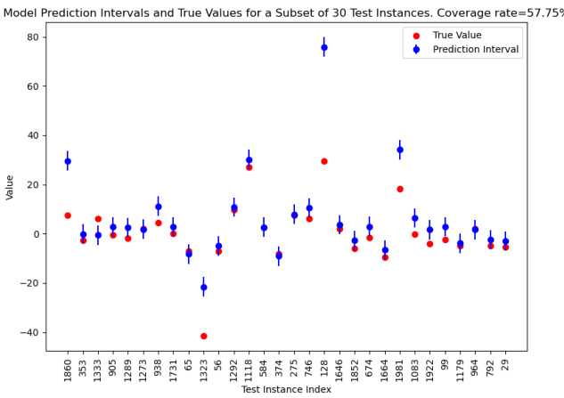
🔼 The figure shows the plug-in model-based predictive intervals and true values for a subset of 30 test instances. The coverage rate is 57.75%. This visualization demonstrates the model’s ability to predict future values within a certain range. The red dots represent true values, and the blue dots with error bars represent prediction intervals generated by the model. The plot is a scatter plot with the x-axis showing test instance indices and the y-axis showing the values (true and predicted). It shows that the prediction intervals tend to be wider, indicating a higher uncertainty around predictions, which is a common trend in prediction tasks.
read the caption
Figure 8: Plug-in model-based predictive interval and coverage.

🔼 This figure shows the results of model-free uncertainty quantification using conformal prediction. The plot displays model prediction intervals and true values for a subset of 30 test instances. A key result is the 95.3% coverage rate, indicating that the true values fall within the predicted intervals in 95.3% of the cases. This demonstrates the effectiveness of conformal prediction compared to the model-based approach (Figure 8).
read the caption
Figure 9: Conformal prediction predictive interval and coverage.
Full paper#


