TL;DR#
Continuous attractor networks are popular theoretical models for analog memory in neuroscience. However, a major challenge is their inherent fragility: small changes to the system destroy the continuous attractor. This paper investigates the robustness of continuous attractors by studying bifurcations and approximations in various theoretical models and recurrent neural networks (RNNs). It highlights the critical weakness of pure continuous attractors and their vulnerability to perturbations.
The researchers use persistent manifold theory and fast-slow decomposition analysis to demonstrate the existence of a structurally stable slow manifold that persists even after bifurcations. This manifold approximates the original continuous attractor, bounding memory errors. They train RNNs on analog memory tasks, verifying that these approximate continuous attractors appear as natural solutions, showing functional robustness, and generalizing well. This study provides a critical theoretical basis and empirical evidence supporting the continued utility of continuous attractors as a framework for understanding analog memory in biological systems.
Key Takeaways#
Why does it matter?#
This paper is crucial for researchers in neuroscience and neural networks. It provides a theoretical framework and experimental evidence to understand the robustness of continuous attractor networks, which are fundamental models for analog memory. The work bridges theoretical neuroscience with practical implementations, offering valuable insights into the design and interpretation of RNNs for analog memory tasks. It opens new avenues for research into the approximation of continuous attractors and their generalization capabilities.
Visual Insights#

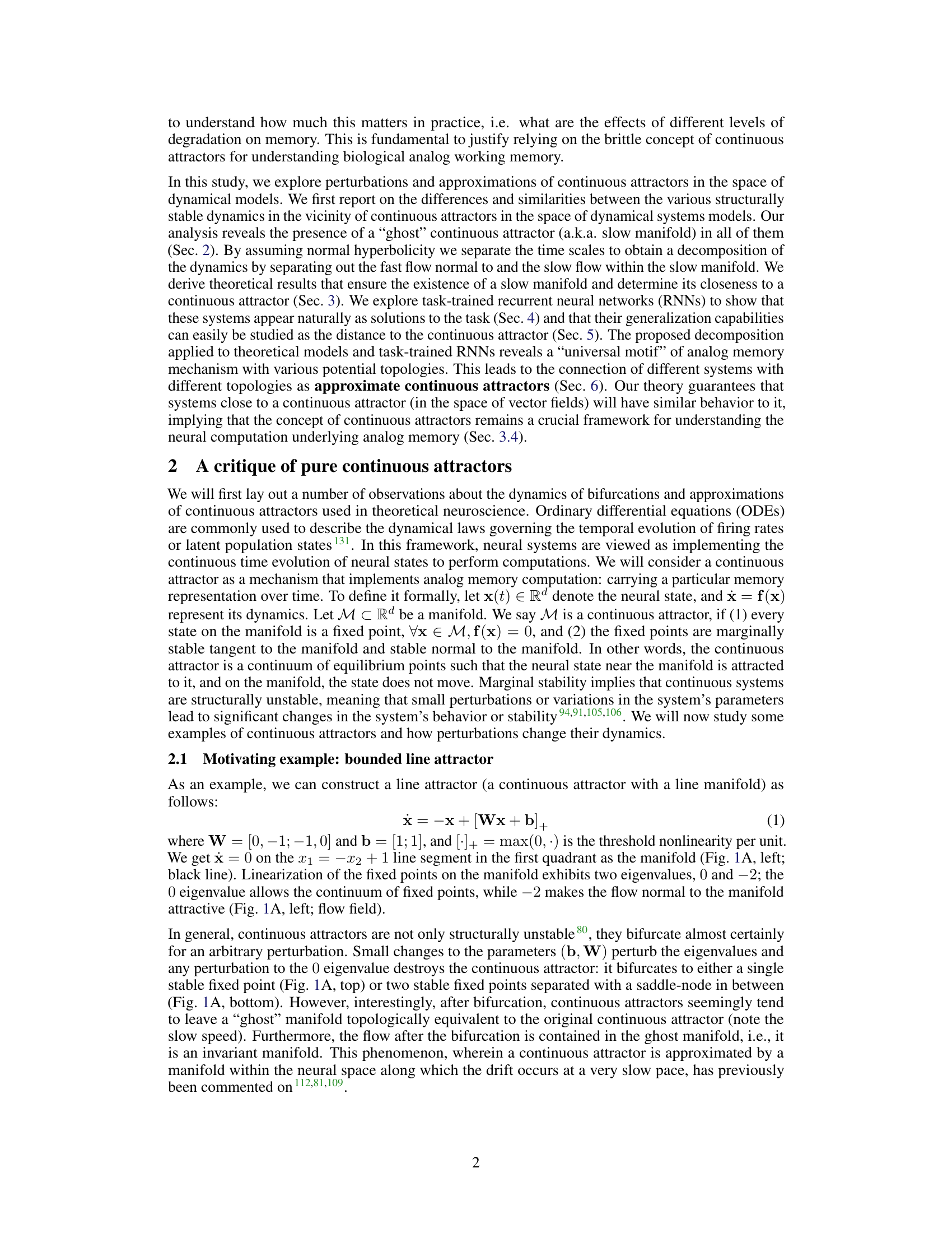
🔼 This figure shows the fragility of continuous attractors and how they can be approximated by structurally stable dynamics. Panel A illustrates the bifurcations of a bounded line attractor under parameter perturbations, demonstrating that even small changes can destroy the continuous attractor. However, a topologically equivalent invariant manifold persists. Panel B shows different topologies that emerge from approximations of ring attractors. These approximations, though not strictly continuous attractors, exhibit similar finite-time behaviors and contain ring-like invariant sets.
read the caption
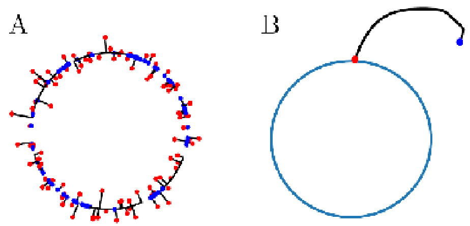
Figure 1: The critical weakness of continuous attractors is their inherent brittleness as they are rare in the parameter space, i.e., infinitesimal changes in parameters destroy the continuous attractor implemented in RNNs 111,103. Some of the structure seems to remain; there is an invariant manifold that is topologically equivalent to the original continuous attractor. (A) Phase portraits for the bounded line attractor (Eq. (1)). Under perturbation of parameters, it bifurcates to systems without the continuous attractor. (B) The low-rank ring attractor approximation (Sec. (S3.4)). Different topologies exist for different realizations of a low-rank attractor: different numbers of fixed points (4, 8, 12), or a limit cycle (right bottom). Yet, they all share the existence of a ring invariant set.

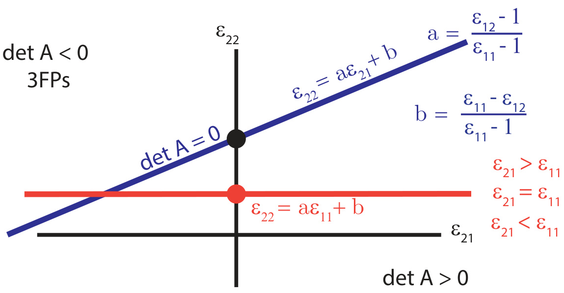
🔼 This table summarizes the conditions under which different bifurcations (1FP (full), 1FP (partial), 3FPs, 2FPs, LA) occur in the bounded line attractor model. C1 and C2 represent two different sets of conditions. A checkmark indicates that the condition is met for that bifurcation type, while an ‘X’ indicates it is not. ‘only Eq22 or 23’ indicates that a specific equation or set of equations must be satisfied for that bifurcation to occur.
read the caption
Table 1: Summary of the conditions for the different bifurcations.
In-depth insights#
Analog Memory#
The paper explores the concept of analog memory, focusing on continuous attractor neural networks as a theoretical model. It critiques the structural instability of pure continuous attractors, highlighting their susceptibility to perturbations. The core argument revolves around the observation that while continuous attractors themselves are fragile, their approximations maintain functionality due to the existence of a persistent slow manifold. This manifold preserves the topological structure of the attractor, ensuring that the system continues to perform analog memory tasks, albeit with potential error that is related to the size of the perturbation. The research combines theoretical analysis of dynamical systems with experimental results from training recurrent neural networks on analog memory tasks, confirming that these networks naturally exhibit this approximate continuous attractor behavior. The study provides a framework for understanding the robustness and resilience of analog memory in biological systems and offers a unifying theoretical explanation for various experimental findings.
Attractor Robustness#
The concept of attractor robustness is central to understanding the reliability of continuous attractor networks (CANs) as models of neural computation. CANs, while theoretically elegant, are notoriously fragile, easily disrupted by small parameter changes or noise. The paper challenges this view, arguing that functional robustness can be achieved even with systems that deviate from the idealized CAN model. This is achieved through the persistent manifold theory, highlighting that even after bifurcation, a slow manifold resembling the original attractor persists. This slow manifold, while not strictly a continuous attractor, maintains analog information over behaviorally relevant timescales, supporting robust memory despite perturbations. The paper provides theoretical arguments and experimental evidence from recurrent neural networks (RNNs) trained on analog memory tasks, demonstrating that approximate continuous attractors are not only plausible but potentially universal motifs for analog memory in biological systems.
RNN Experiments#
The RNN experiments section evaluates the performance of recurrent neural networks (RNNs) on analog memory tasks. The authors trained various RNN architectures (vanilla RNNs with different activation functions, LSTMs, and GRUs) on tasks requiring the storage and retrieval of continuous variables like head direction. A key finding is the emergence of approximate continuous attractors, structures that are not perfect mathematical continuous attractors but functionally resemble them by confining dynamics to a slow manifold. This suggests that biological systems might employ similar approximations rather than the idealized continuous attractors often proposed in theoretical models. The analysis focused on the generalization properties of different topological solutions (fixed points, limit cycles), providing evidence for the functional robustness of approximate continuous attractors and their relevance for understanding analog memory in biological systems. Crucially, the authors demonstrate the link between the topology of these approximate attractors and their generalization capabilities. This deep dive into the relationship between network dynamics, task performance, and generalization helps bridge the gap between theoretical models and experimental observations of neural activity during working memory tasks.
Manifold Theory#
Manifold theory, in the context of this research paper, offers a powerful framework for analyzing the robustness of continuous attractor networks in the face of perturbations. The core idea is that despite the inherent fragility of continuous attractors, a slow invariant manifold persists even after bifurcations, essentially acting as a ‘ghost’ attractor. This manifold, closely resembling the original continuous attractor in topology, maintains the system’s ability to store continuous-valued information. The theory provides a mathematical basis for understanding this robustness by separating timescales (fast flow normal to the manifold, slow flow within), and enabling the bounding of memory errors based on the manifold’s dynamics. Normal hyperbolicity of the manifold is a crucial condition ensuring persistence and stability. The application of manifold theory offers valuable insights into the functional resilience of continuous attractor neural networks for analog memory and provides a theoretical grounding for future investigations into biological neural systems.
Future Research#
Future research directions stemming from this work could explore several promising avenues. Extending the theoretical framework to encompass non-compact manifolds and more complex topologies would enhance applicability to real-world systems. Investigating the impact of different types of noise beyond those examined here, such as correlated noise or noise affecting specific network parameters, is crucial to understand robustness in realistic scenarios. Experimentally validating the predicted relationship between the speed of flow on the slow manifold and memory performance would provide strong empirical support. Finally, exploring the role of learning and plasticity in shaping and maintaining approximate continuous attractors could reveal insights into the brain’s remarkable capacity for flexible analog memory.
More visual insights#
More on figures

🔼 This figure shows the results of perturbing different implementations of ring attractors. Each subfigure shows a different model of a ring attractor after various perturbations. Despite these perturbations, a ring-like structure (the invariant manifold) remains in all cases. The nodes in the ring are either stable fixed points or saddle points. (A) Shows the results for a specific ring attractor model from the literature. (B) Shows the effect on a tanh approximation of a ring attractor. (C) Shows the effects of perturbations on approximate ring attractors generated using Embedding Manifolds with Population-level Jacobians (EMPJ).
read the caption
Figure 2: Perturbations of different implementations and approximations of ring attractors lead to bifurcations that all leave the ring invariant manifold intact. For each model, the network dynamics is constrained to a ring which in turn is populated by stable fixed points (green) and saddle nodes (red). (A) Perturbations to the ring attractor88. The ring attractor can be perturbed in systems with an even number of fixed points (FPs) up to 2N (stable and saddle points are paired). (B) Perturbations to a tanh approximation of a ring attractor110. (C) Different Embedding Manifolds with Population-level Jacobians (EMPJ) approximations of a ring attractor96.

🔼 This figure illustrates the Persistent Manifold Theorem. The left panel shows a continuous attractor (M₀), a manifold of equilibria where the flow is zero. The right panel shows what happens after a small perturbation (ε). The continuous attractor is destroyed, but a persistent slow manifold (Mε) emerges. This manifold has the same topology as the original continuous attractor, and the flow is still attractive, meaning trajectories are drawn to and remain within the manifold. The dashed line represents a trajectory that remains trapped on the slow manifold. This illustrates how, despite the disappearance of the continuous attractor, its functional properties are preserved in the form of a persistent slow manifold.
read the caption
Figure 3: Persistent manifold theorem applied to compact continuous attractor guarantees the flow on the slow manifold Mε is invariant and continues to be attractive. The dashed line is a trajectory “trapped” in the slow manifold (which has the same topology as the continuous attractor).
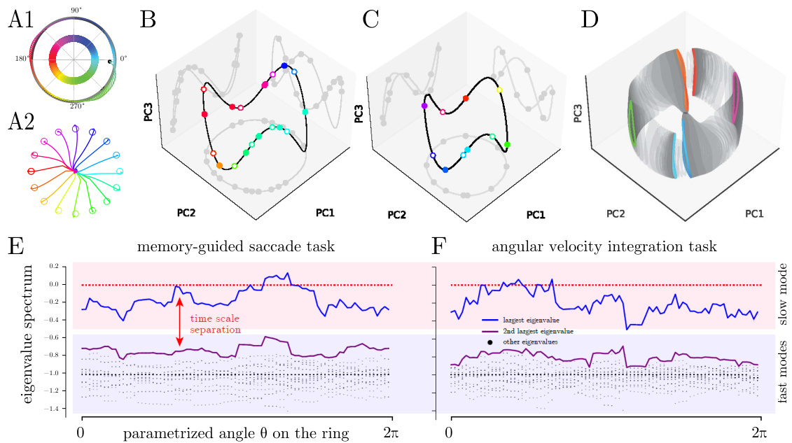
🔼 This figure displays the results of training recurrent neural networks (RNNs) on two different tasks: a memory-guided saccade task and an angular velocity integration task. The figure shows the slow manifold approximation of different trained networks on these tasks, illustrating various topologies such as fixed-point rings, limit cycles, and a slow torus. The eigenvalue spectra for selected networks demonstrate a time scale separation, indicative of normal hyperbolicity.
read the caption
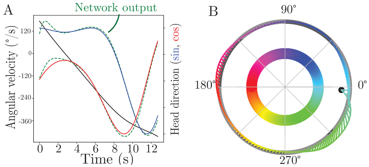
Figure 4: Slow manifold approximation of different trained networks on the memory-guided saccade and angular velocity integration tasks. (A1) Output of an example trajectory on the angular velocity integration task. (A2) Output of a example trajectories on the memory-guided saccade task. (B) An example fixed-point type solution to the memory-guided saccade task. Circles indicate fixed points of the system (filled for stable, empty for saddle) and the decoded angular value on the output ring is indicated with the color according to A1. (C) An example of a found solution to the angular velocity integration task. (D) An example slow-torus type solution to the memory-guided saccade task. The colored curves indicate stable limit cycles of the system. (E+F) The eigenvalue spectrum for the trained networks in B and C show a gap between the first two largest eigenvalues.

🔼 This figure shows the relationship between different measures of memory capacity and generalization performance of trained recurrent neural networks (RNNs). Panel A shows the relationship between average angular error and the uniform norm of the vector field for both finite and asymptotic timescales. Panel B plots the memory capacity against the average angular error. Panel C illustrates the relationship between the average angular error and the number of fixed points in the network, with the average distance between neighboring fixed points highlighted in magenta. Panel D presents the time course of average angular error for two specific networks. Finally, Panel E shows the distribution of network performance, measured as normalized mean squared error (NMSE), on a validation dataset.
read the caption
Figure 5: The different measures for memory capacity reflect the generalization properties implied by the topology of the found solution. (A) The average accumulated angular error versus the uniform norm on the vector field (left and right hand side of Eq. 5, respectively), shown for finite time (time of trial length on which networks were trained, T₁) indicated with filled markers and at asymptotic time (with hollow markers). (B) The memory capacity versus the average accumulated angular error. (C) The number of fixed points versus average accumulated angular error, with the average distance between neighboring fixed points indicated in magenta. (D) The average accumulated angular error over time for two selected networks, indicated with the blue and orange arrows in (C). (E) Distribution of network performance measured on a validation dataset measured as normalized MSE (NMSE).
🔼 This figure demonstrates the fragility of continuous attractors and how they are affected by small changes in parameters. Panel A illustrates phase portraits for a bounded line attractor, showing how bifurcations lead to systems without continuous attractors, while still preserving a topologically equivalent invariant manifold. Panel B illustrates the different topologies found for low-rank ring attractor approximations, exhibiting various numbers of fixed points or even a limit cycle, all with a common ring-like invariant structure.
read the caption
Figure 1: The critical weakness of continuous attractors is their inherent brittleness as they are rare in the parameter space, i.e., infinitesimal changes in parameters destroy the continuous attractor implemented in RNNs 111,103. Some of the structure seems to remain; there is an invariant manifold that is topologically equivalent to the original continuous attractor. (A) Phase portraits for the bounded line attractor (Eq. (1)). Under perturbation of parameters, it bifurcates to systems without the continuous attractor. (B) The low-rank ring attractor approximation (Sec. (S3.4)). Different topologies exist for different realizations of a low-rank attractor: different numbers of fixed points (4, 8, 12), or a limit cycle (right bottom). Yet, they all share the existence of a ring invariant set.

🔼 This figure shows the critical weakness of continuous attractors, which is their inherent brittleness due to their rarity in the parameter space. Infinitesimal changes in parameters can destroy them. However, some structure seems to remain, as an invariant manifold that is topologically equivalent to the original continuous attractor. Panel (A) displays phase portraits for the bounded line attractor, illustrating bifurcations under parameter perturbations. Panel (B) shows different topologies resulting from the low-rank ring attractor approximation, ranging from different numbers of fixed points to a limit cycle, highlighting the existence of a ring invariant set in all cases.
read the caption
Figure 1: The critical weakness of continuous attractors is their inherent brittleness as they are rare in the parameter space, i.e., infinitesimal changes in parameters destroy the continuous attractor implemented in RNNs 111,103. Some of the structure seems to remain; there is an invariant manifold that is topologically equivalent to the original continuous attractor. (A) Phase portraits for the bounded line attractor (Eq. (1)). Under perturbation of parameters, it bifurcates to systems without the continuous attractor. (B) The low-rank ring attractor approximation (Sec. (S3.4)). Different topologies exist for different realizations of a low-rank attractor: different numbers of fixed points (4, 8, 12), or a limit cycle (right bottom). Yet, they all share the existence of a ring invariant set.

🔼 This figure shows how different implementations of ring attractors respond to perturbations. Despite the perturbations causing bifurcations, a ring-shaped invariant manifold remains. Panel A shows perturbations to a specific ring attractor model, demonstrating a change in the number of fixed points but the persistence of the ring structure. Panel B shows similar results for a tanh approximation of a ring attractor. Panel C illustrates the same phenomenon for ring attractors approximated using the Embedding Manifolds with Population-level Jacobians (EMPJ) method.
read the caption
Figure 2: Perturbations of different implementations and approximations of ring attractors lead to bifurcations that all leave the ring invariant manifold intact. For each model, the network dynamics is constrained to a ring which in turn is populated by stable fixed points (green) and saddle nodes (red). (A) Perturbations to the ring attractor88. The ring attractor can be perturbed in systems with an even number of fixed points (FPs) up to 2N (stable and saddle points are paired). (B) Perturbations to a tanh approximation of a ring attractor110. (C) Different Embedding Manifolds with Population-level Jacobians (EMPJ) approximations of a ring attractor96.
🔼 This figure displays the generalization capabilities of recurrent neural networks trained on an angular velocity integration task. The networks’ performance is assessed using different metrics: average accumulated angular error (related to the uniform norm of the vector field), memory capacity (entropy), and the number of fixed points. Panel (A) compares the angular error for both short and long time scales, revealing the relationship between error and the uniform norm. Panel (B) examines the trade-off between memory capacity and error. Panel (C) shows how the number of fixed points affects error, with additional information on the average distance between fixed points. Panel (D) demonstrates error over time for specific networks. Finally, Panel (E) provides a distribution of network performance using normalized MSE.
read the caption
Figure 5: The different measures for memory capacity reflect the generalization properties implied by the topology of the found solution. (A) The average accumulated angular error versus the uniform norm on the vector field (left and right hand side of Eq. 5, respectively), shown for finite time (time of trial length on which networks were trained, T₁) indicated with filled markers and at asymptotic time (with hollow markers). (B) The memory capacity versus the average accumulated angular error. (C) The number of fixed points versus average accumulated angular error, with the average distance between neighboring fixed points indicated in magenta. (D) The average accumulated angular error over time for two selected networks, indicated with the blue and orange arrows in (C). (E) Distribution of network performance measured on a validation dataset measured as normalized MSE (NMSE).

🔼 This figure shows the results of perturbing different implementations of ring attractors. Panel A shows perturbations of a piecewise-linear ring attractor model (from the fruit fly head direction system). Panel B shows perturbations of a ring attractor model approximated using tanh neurons. Panel C shows perturbations of ring attractors approximated using the Embedding Manifolds with Population-level Jacobians (EMPJ) method. In all cases, the perturbations lead to bifurcations that change the number of fixed points, but the ring-like invariant manifold remains intact. The fixed points are colored green for stable and red for saddle.
read the caption
Figure 2: Perturbations of different implementations and approximations of ring attractors lead to bifurcations that all leave the ring invariant manifold intact. For each model, the network dynamics is constrained to a ring which in turn is populated by stable fixed points (green) and saddle nodes (red). (A) Perturbations to the ring attractor88. The ring attractor can be perturbed in systems with an even number of fixed points (FPs) up to 2N (stable and saddle points are paired). (B) Perturbations to a tanh approximation of a ring attractor110. (C) Different Embedding Manifolds with Population-level Jacobians (EMPJ) approximations of a ring attractor96.
🔼 This figure illustrates the brittleness of continuous attractors and how they are affected by perturbations. Panel A shows phase portraits for a bounded line attractor, demonstrating how small parameter changes lead to bifurcations, destroying the continuous attractor but leaving a topologically equivalent invariant manifold. Panel B shows approximations of low-rank ring attractors, highlighting various topologies resulting from different realizations (4, 8, 12 fixed points or a limit cycle). Despite the topological differences, all approximations share a common ring invariant set.
read the caption
Figure 1: The critical weakness of continuous attractors is their inherent brittleness as they are rare in the parameter space, i.e., infinitesimal changes in parameters destroy the continuous attractor implemented in RNNs 111,103. Some of the structure seems to remain; there is an invariant manifold that is topologically equivalent to the original continuous attractor. (A) Phase portraits for the bounded line attractor (Eq. (1)). Under perturbation of parameters, it bifurcates to systems without the continuous attractor. (B) The low-rank ring attractor approximation (Sec. (S3.4)). Different topologies exist for different realizations of a low-rank attractor: different numbers of fixed points (4, 8, 12), or a limit cycle (right bottom). Yet, they all share the existence of a ring invariant set.

🔼 This figure shows how different implementations of ring attractors respond to perturbations. Each subfigure (A, B, C) displays a different model of a ring attractor, illustrating how the system’s dynamics remain constrained to a ring-shaped invariant manifold even after perturbation. This manifold is populated by stable fixed points (green) and saddle nodes (red). The subfigures highlight that while the specific number of fixed points varies depending on the model and the perturbation, the underlying ring structure remains persistent. This suggests that systems close to a continuous attractor still maintain the ring-like structure in their dynamics.
read the caption
Figure 2: Perturbations of different implementations and approximations of ring attractors lead to bifurcations that all leave the ring invariant manifold intact. For each model, the network dynamics is constrained to a ring which in turn is populated by stable fixed points (green) and saddle nodes (red). (A) Perturbations to the ring attractor 88. The ring attractor can be perturbed in systems with an even number of fixed points (FPs) up to 2N (stable and saddle points are paired). (B) Perturbations to a tanh approximation of a ring attractor110. (C) Different Embedding Manifolds with Population-level Jacobians (EMPJ) approximations of a ring attractor 96.

🔼 This figure demonstrates that perturbations to different types of ring attractors (continuous attractors with a ring topology) result in bifurcations that preserve a ring-like invariant manifold. The figure shows phase portraits for three different models of ring attractors: (A) a biologically-inspired model of the central complex of fruit flies; (B) an approximation using tanh neurons; and (C) an approximation using the EMPJ method. In each case, the original ring attractor is perturbed, leading to bifurcations that either create an even number of fixed points (stable and saddle points paired) or alter the number of fixed points. Despite these bifurcations, the topology of the system remains largely unchanged, with activity still confined to an invariant manifold resembling the original ring.
read the caption
Figure 2: Perturbations of different implementations and approximations of ring attractors lead to bifurcations that all leave the ring invariant manifold intact. For each model, the network dynamics is constrained to a ring which in turn is populated by stable fixed points (green) and saddle nodes (red). (A) Perturbations to the ring attractor88. The ring attractor can be perturbed in systems with an even number of fixed points (FPs) up to 2N (stable and saddle points are paired). (B) Perturbations to a tanh approximation of a ring attractor110. (C) Different Embedding Manifolds with Population-level Jacobians (EMPJ) approximations of a ring attractor96.
🔼 This figure presents a comparison of slow manifold approximations obtained from different recurrent neural networks (RNNs) trained on two distinct tasks: a memory-guided saccade task and an angular velocity integration task. Subfigures A1 and A2 show example trajectories for each task. Subfigures B, C, and D illustrate different types of solutions found by the RNNs, specifically showing fixed points (B), limit cycles (C), and slow-torus dynamics (D). Subfigures E and F display the eigenvalue spectrums for two of these networks (B and C) and highlight the characteristic time-scale separation associated with normally hyperbolic invariant manifolds.
read the caption
Figure 4: Slow manifold approximation of different trained networks on the memory-guided saccade and angular velocity integration tasks. (A1) Output of an example trajectory on the angular velocity integration task. (A2) Output of a example trajectories on the memory-guided saccade task. (B) An example fixed-point type solution to the memory-guided saccade task. Circles indicate fixed points of the system (filled for stable, empty for saddle) and the decoded angular value on the output ring is indicated with the color according to A1. (C) An example of a found solution to the angular velocity integration task. (D) An example slow-torus type solution to the memory-guided saccade task. The colored curves indicate stable limit cycles of the system. (E+F) The eigenvalue spectrum for the trained networks in B and C show a gap between the first two largest eigenvalues.

🔼 This figure shows the slow manifold approximation for four different trained RNNs on two different tasks. The top panels show example trajectories for each task (A1 and A2), illustrating the dynamics. The middle panels (B, C, D) display the resulting slow manifold structure after training – panels B and C show fixed-point type solutions and panel D shows a slow-torus solution. The bottom panels (E and F) show the eigenvalue spectrum for two networks (B and C), illustrating the time scale separation indicating the presence of a persistent slow manifold.
read the caption
Figure 4: Slow manifold approximation of different trained networks on the memory-guided saccade and angular velocity integration tasks. (A1) Output of an example trajectory on the angular velocity integration task. (A2) Output of a example trajectories on the memory-guided saccade task. (B) An example fixed-point type solution to the memory-guided saccade task. Circles indicate fixed points of the system (filled for stable, empty for saddle) and the decoded angular value on the output ring is indicated with the color according to A1. (C) An example of a found solution to the angular velocity integration task. (D) An example slow-torus type solution to the memory-guided saccade task. The colored curves indicate stable limit cycles of the system. (E+F) The eigenvalue spectrum for the trained networks in B and C show a gap between the first two largest eigenvalues.

🔼 This figure shows different ways to measure the memory capacity of recurrent neural networks trained to perform analog memory tasks. Panel A compares the average angular error at different timescales (training duration and asymptotically) to the speed of the network’s dynamics on the slow manifold, showing a linear relationship. Panel B connects memory capacity (entropy) to the accumulated error. Panel C relates the number of fixed points on the slow manifold (and distance between them) to the error. Panel D shows the time evolution of error for selected examples, and panel E displays a distribution of normalized MSE scores across the tested networks.
read the caption
Figure 5: The different measures for memory capacity reflect the generalization properties implied by the topology of the found solution. (A) The average accumulated angular error versus the uniform norm on the vector field (left and right hand side of Eq. 5, respectively), shown for finite time (time of trial length on which networks were trained, T₁) indicated with filled markers and at asymptotic time (with hollow markers). (B) The memory capacity versus the average accumulated angular error. (C) The number of fixed points versus average accumulated angular error, with the average distance between neighboring fixed points indicated in magenta. (D) The average accumulated angular error over time for two selected networks, indicated with the blue and orange arrows in (C). (E) Distribution of network performance measured on a validation dataset measured as normalized MSE (NMSE).

🔼 This figure shows the results of training recurrent neural networks on two different tasks: a memory-guided saccade task and an angular velocity integration task. It displays the slow manifolds found in the trained networks, which approximate continuous attractors. Different network architectures and activation functions lead to distinct manifold topologies (fixed points, limit cycles). The eigenvalue spectra demonstrate that these topologies exhibit fast-slow dynamics, suggesting normal hyperbolicity.
read the caption
Figure 4: Slow manifold approximation of different trained networks on the memory-guided saccade and angular velocity integration tasks. (A1) Output of an example trajectory on the angular velocity integration task. (A2) Output of a example trajectories on the memory-guided saccade task. (B) An example fixed-point type solution to the memory-guided saccade task. Circles indicate fixed points of the system (filled for stable, empty for saddle) and the decoded angular value on the output ring is indicated with the color according to A1. (C) An example of a found solution to the angular velocity integration task. (D) An example slow-torus type solution to the memory-guided saccade task. The colored curves indicate stable limit cycles of the system. (E+F) The eigenvalue spectrum for the trained networks in B and C show a gap between the first two largest eigenvalues.

🔼 This figure displays the relationship between different measures of memory capacity and generalization performance of trained recurrent neural networks (RNNs). Panel A shows the average accumulated angular error versus the uniform norm of the vector field for both finite and asymptotic timescales. Panel B shows the relationship between memory capacity and average angular error. Panel C shows the number of fixed points, their average distance, and angular error. Panel D illustrates the angular error over time for two specific networks. Finally, Panel E shows the distribution of network performance on a validation dataset.
read the caption
Figure 5: The different measures for memory capacity reflect the generalization properties implied by the topology of the found solution. (A) The average accumulated angular error versus the uniform norm on the vector field (left and right hand side of Eq. 5, respectively), shown for finite time (time of trial length on which networks were trained, T₁) indicated with filled markers and at asymptotic time (with hollow markers). (B) The memory capacity versus the average accumulated angular error. (C) The number of fixed points versus average accumulated angular error, with the average distance between neighboring fixed points indicated in magenta. (D) The average accumulated angular error over time for two selected networks, indicated with the blue and orange arrows in (C). (E) Distribution of network performance measured on a validation dataset measured as normalized MSE (NMSE).

🔼 This figure shows that perturbations to different types of ring attractors all leave the ring-shaped invariant manifold intact, although the specific dynamics (number of fixed points, limit cycles) may change. Panel A shows the bifurcations of a biologically-inspired ring attractor model; panel B shows the bifurcations of a tanh approximation; and panel C shows the bifurcations of a ring attractor approximated using the Embedding Manifolds with Population-level Jacobians (EMPJ) method. In all cases, the invariant manifold remains a ring-like structure, indicating robustness of the underlying topology.
read the caption
Figure 2: Perturbations of different implementations and approximations of ring attractors lead to bifurcations that all leave the ring invariant manifold intact. For each model, the network dynamics is constrained to a ring which in turn is populated by stable fixed points (green) and saddle nodes (red). (A) Perturbations to the ring attractor 88. The ring attractor can be perturbed in systems with an even number of fixed points (FPs) up to 2N (stable and saddle points are paired). (B) Perturbations to a tanh approximation of a ring attractor110. (C) Different Embedding Manifolds with Population-level Jacobians (EMPJ) approximations of a ring attractor 96.
🔼 This figure shows various ways of measuring the performance of the trained recurrent neural networks on an angular velocity integration task. Panel A compares the average angular error at different time scales with the uniform norm of the vector field on the manifold, illustrating how network performance degrades over longer time scales. Panel B compares memory capacity (entropy) with the average accumulated angular error, providing another perspective on generalization. Panel C shows a relationship between the number of fixed points in the network and the average error. Panel D depicts the error over time for two selected networks. Finally, Panel E displays the distribution of normalized mean squared error (NMSE) across the trained networks.
read the caption
Figure 5: The different measures for memory capacity reflect the generalization properties implied by the topology of the found solution. (A) The average accumulated angular error versus the uniform norm on the vector field (left and right hand side of Eq. 5, respectively), shown for finite time (time of trial length on which networks were trained, T₁) indicated with filled markers and at asymptotic time (with hollow markers). (B) The memory capacity versus the average accumulated angular error. (C) The number of fixed points versus average accumulated angular error, with the average distance between neighboring fixed points indicated in magenta. (D) The average accumulated angular error over time for two selected networks, indicated with the blue and orange arrows in (C). (E) Distribution of network performance measured on a validation dataset measured as normalized MSE (NMSE).

🔼 This figure shows the results of training recurrent neural networks (RNNs) on two different tasks: memory-guided saccade and angular velocity integration. Panels A1 and A2 display example trajectories. Panels B, C, and D illustrate different types of solutions discovered by the RNNs, characterized by their dynamics: fixed-point ring manifold, limit cycle and slow torus. The solutions are not pure continuous attractors, but rather approximations exhibiting slow manifolds, whose existence is supported by the eigenvalue spectrum displayed in Panels E and F.
read the caption
Figure 4: Slow manifold approximation of different trained networks on the memory-guided saccade and angular velocity integration tasks. (A1) Output of an example trajectory on the angular velocity integration task. (A2) Output of a example trajectories on the memory-guided saccade task. (B) An example fixed-point type solution to the memory-guided saccade task. Circles indicate fixed points of the system (filled for stable, empty for saddle) and the decoded angular value on the output ring is indicated with the color according to A1. (C) An example of a found solution to the angular velocity integration task. (D) An example slow-torus type solution to the memory-guided saccade task. The colored curves indicate stable limit cycles of the system. (E+F) The eigenvalue spectrum for the trained networks in B and C show a gap between the first two largest eigenvalues.
Full paper#

