↗ OpenReview ↗ NeurIPS Homepage ↗ Chat
TL;DR#
Black-box optimization (BBO) is crucial yet challenging, especially in zero-shot scenarios where optimizers must adapt to unseen tasks. Existing methods often struggle, requiring intricate hyperparameter tuning. This necessitates efficient, robust optimization methods capable of generalizing across diverse tasks.
This paper introduces the Pretrained Optimization Model (POM), addressing this challenge by leveraging knowledge from various tasks to offer efficient zero-shot solutions. POM’s performance is evaluated on the BBOB benchmark and robot control tasks, showcasing superior performance, particularly for high-dimensional tasks. Fine-tuning with a small number of samples yields significant performance improvements, demonstrating robust generalization.
Key Takeaways#
Why does it matter?#
This paper is important because it introduces POM, a novel approach to zero-shot black-box optimization that outperforms state-of-the-art methods, especially for high-dimensional problems. This has significant implications for various fields relying on efficient optimization, opening new avenues for research in meta-learning and robust optimization strategies. The MetaGBT training method ensures rapid and stable training of the model, and the demonstrated robust generalization makes it valuable for diverse applications.
Visual Insights#

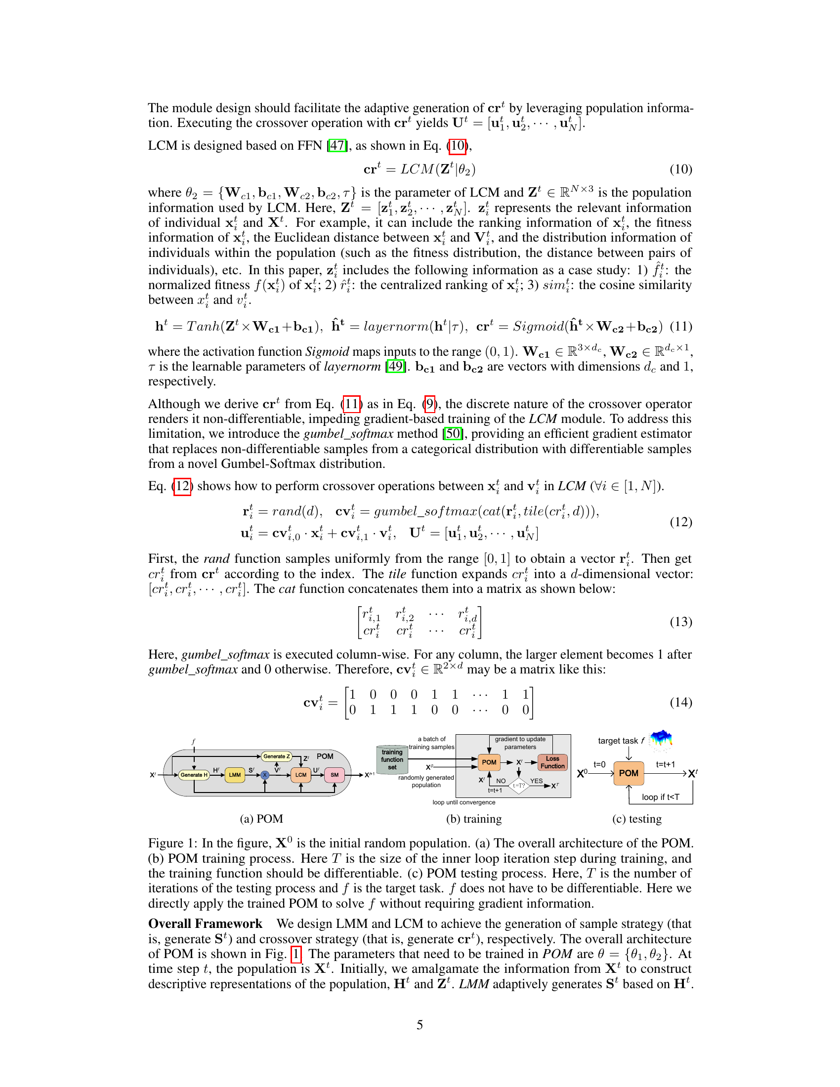
This figure illustrates the architecture of the Pretrained Optimization Model (POM), its training process, and its testing process. The architecture diagram (a) shows the flow of data through the LMM (Learned Mutation Module), LCM (Learned Crossover Module), and SM (Selection Module) components of the POM. The training process (b) highlights how the POM is trained using a set of training functions, a differentiable loss function, and gradient-based optimization. This training process fine-tunes the POM parameters. The testing process (c) demonstrates how the trained POM can be directly applied to an unseen target task to find an optimal solution without requiring gradient information. The training process utilizes the gradient to update the parameters until convergence, whereas the testing process involves iterative steps to achieve the optimal solution.
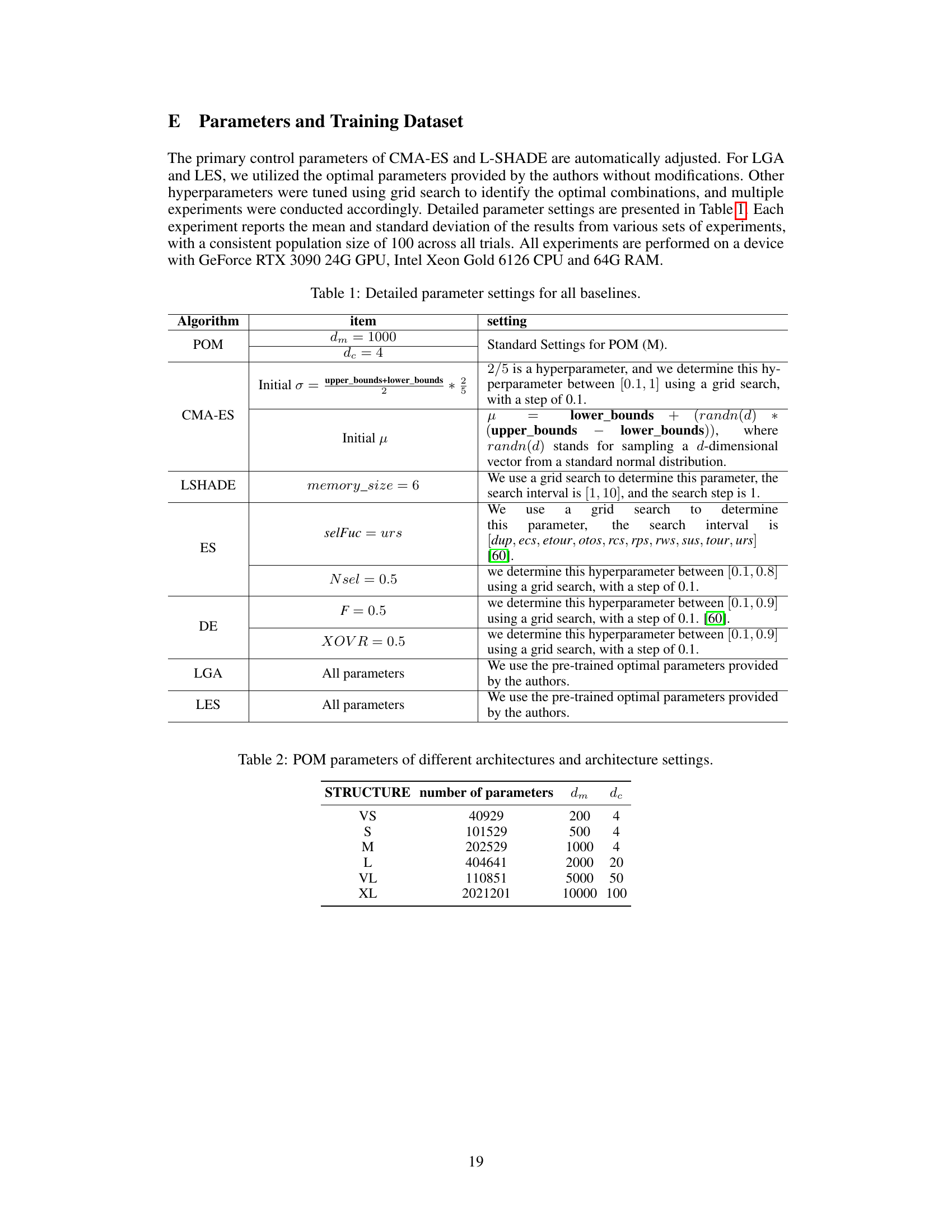
This table lists the detailed parameter settings used for all baseline algorithms in the experiments, including CMA-ES, L-SHADE, ES, DE, LGA, and LES. It provides specific values for hyperparameters, initial values, and settings crucial for the reproducibility of the experimental results. Note that for some algorithms (CMA-ES and L-SHADE), parameters were automatically adjusted, while others (LGA and LES) utilized parameters provided by the authors. For algorithms where grid search was used to determine parameters, the search ranges and steps are specified.
In-depth insights#
Zero-Shot Optimization#
Zero-shot optimization presents a significant challenge and opportunity in machine learning. The goal is to develop optimizers capable of tackling unseen tasks without any task-specific hyperparameter tuning or retraining. This is crucial for enhancing the robustness and adaptability of optimization algorithms across diverse applications. Current methods often struggle with zero-shot generalization, necessitating extensive tuning. Pretrained Optimization Models (POMs), as discussed in the provided text, offer a promising approach by leveraging knowledge learned from a diverse set of training tasks. A key advantage of POMs is their ability to generalize effectively to novel tasks with minimal fine-tuning, making them more efficient and practical. The success of POMs hinges on the design of effective training strategies that capture generalizable optimization principles. Robust generalization remains a core area for improvement, and understanding how POMs adapt to different task distributions and dimensions is vital for realizing the full potential of zero-shot optimization. Future research should explore improved training methodologies and explore novel architectural designs to push the boundaries of this important area.
Pretrained POM Model#
The Pretrained Optimization Model (POM) represents a novel approach to zero-shot black-box optimization. Instead of relying on task-specific tuning, POM leverages a pre-training phase across diverse optimization tasks, learning generalizable strategies. This allows the model to efficiently optimize unseen target tasks with minimal or no adaptation, showcasing robustness and efficiency. The core of POM involves a population-based approach that incorporates innovative modules like the Learning Mutation Module (LMM) and the Learning Crossover Module (LCM). These modules dynamically adjust mutation and crossover strategies based on learned information from the population, resulting in enhanced fitness landscape exploration. MetaGBT training further enhances POM’s performance. The results highlight POM’s superiority over state-of-the-art methods in zero-shot settings, particularly for high-dimensional problems. Further investigation into the model’s scalability and robustness across diverse problem domains is warranted.
MetaGBT Training#
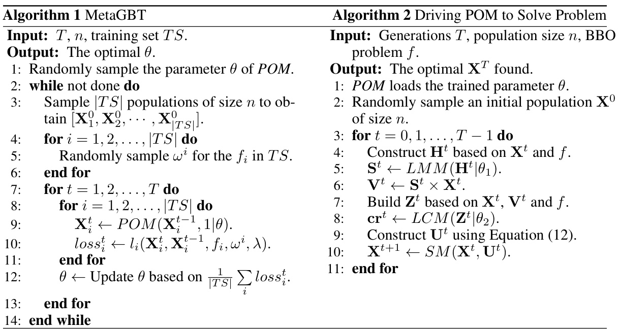
MetaGBT, a meta-gradient-based training framework, is crucial for the Pretrained Optimization Model (POM). It addresses the challenge of training a population-based optimizer on diverse tasks by using an end-to-end gradient-based approach. MetaGBT ensures stable and efficient training of POM, avoiding issues like local optima and overfitting that can arise from sequential task training. By leveraging multiple individuals and diverse tasks, POM acquires a robust and generalizable optimization strategy. The success of MetaGBT lies in its ability to overcome the limitations of other meta-learning methods, particularly those facing issues with parameter explosion and training instability. Its efficiency is crucial for creating a POM capable of zero-shot black-box optimization. This innovative training strategy is fundamental to the performance of POM in solving unseen optimization problems without hyperparameter adjustments.
Ablation Study#
An ablation study systematically removes components of a model to assess their individual contributions. In the context of a black-box optimization model, this involves progressively disabling key modules like the learning module (LMM), crossover module (LCM), or masking mechanism. By comparing the performance of the full model against these variants, researchers can quantify the impact of each module on overall optimization success. The results will highlight the relative importance of various components. Significant performance drops when removing a particular module would strongly suggest that the module is crucial to the algorithm’s success. Conversely, minimal impact might indicate redundancy or areas for potential simplification. A well-executed ablation study is vital for understanding the model’s inner workings, justifying design choices, and identifying potential areas for future improvements. It provides a rigorous test of the model’s robustness and capabilities.
Future Works#
The heading ‘Future Works’ in a research paper typically outlines potential directions for extending the current research. For this specific paper, several promising avenues emerge. Improving the loss function to better balance population convergence and diversity could enhance the algorithm’s robustness and performance. Addressing the computational complexity, especially concerning the attention mechanism’s O(n²) time complexity, is crucial for scaling to larger problems. A thorough investigation into the relationship between model size, training data volume, and training difficulty is warranted, aiming for a more efficient and effective pre-training strategy. Finally, a detailed exploration of the limitations of the proposed approach across diverse scenarios, including different task distributions and dimensions, should be prioritized. Furthermore, exploring the applicability of POM to specific real-world applications, beyond those presented in the paper, and conducting extensive evaluations are suggested. Investigating the transfer learning capabilities of the POM model across different tasks would also provide valuable insights. In addition, a comparison of POM with more recent advanced black-box optimization methods would improve the assessment of its contribution to the field.
More visual insights#
More on figures

This figure shows the results of a critical difference diagram comparing seven algorithms (POM, LSHADE, CMA-ES, LGA, DE, ES, LES) on 24 BBOB problems with dimensions 30 and 100. The Wilcoxon-Holm statistical test (p=0.05) was used to determine statistically significant differences in performance. Higher scores indicate better overall performance across all tested problems.

This figure shows the experimental results for two robot control tasks: Bipedal Walker and Enduro. The y-axis represents the total reward (R) accumulated by the robot during its interaction with the environment. The x-axis represents the generation number. The figure compares the performance of POM against several other algorithms (CMA-ES, DE, ES, LES, LGA, and L-SHADE), demonstrating POM’s superior performance in both tasks, particularly in achieving stable and quick convergence.

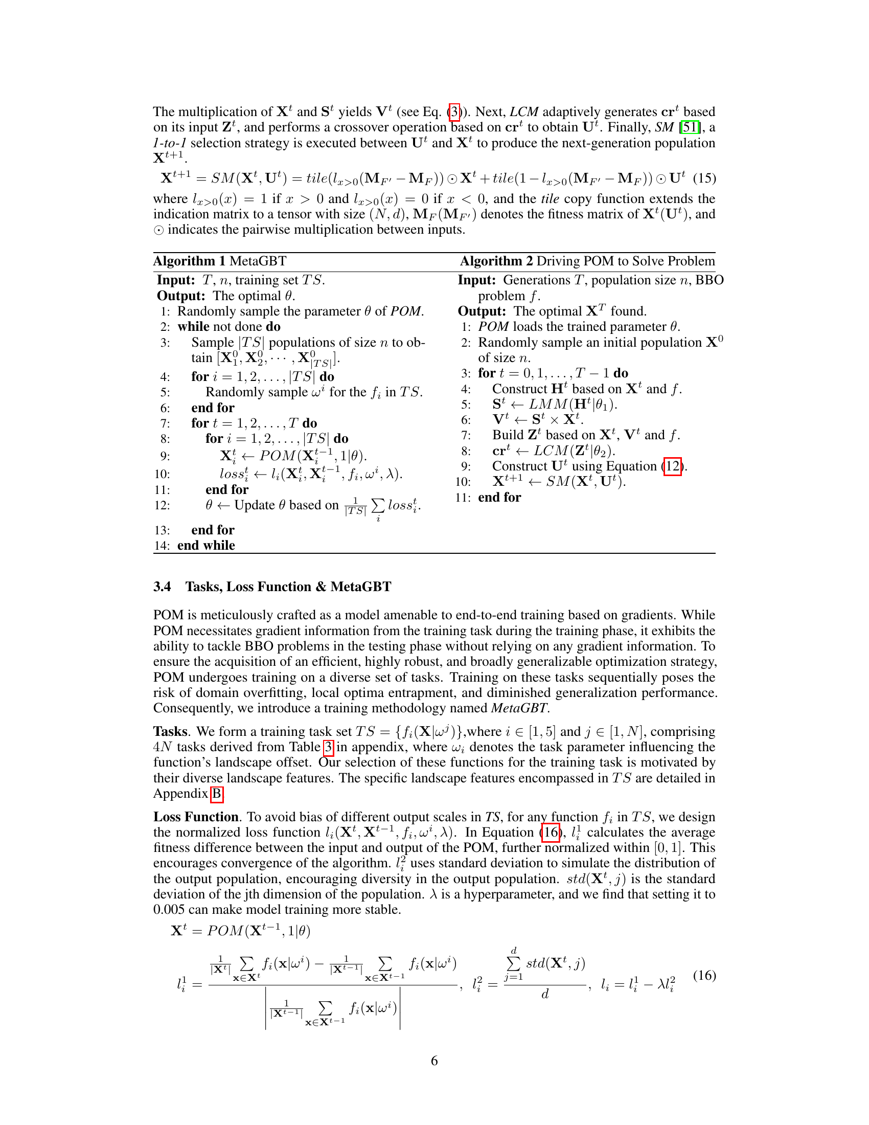
This figure presents the ablation study results for the proposed Pretrained Optimization Model (POM) and shows the impact of different components on the performance. (a) shows the ablation study results using four different configurations: UNTRAINED (untrained model), NO LMM (without the LMM module), NO LCM (without the LCM module), and NO MASK (without the mask operation). The metric used is the optimal function value, with smaller values indicating better performance. (b) shows the results of POMs with different population sizes tested on the BBOB benchmark with dimensions d = 100. The study shows that all components of POM contribute significantly to the model’s performance.

This figure presents the ablation study and the impact of different sizes of POM on BBOB test performance. (a) shows the performance of POM compared to versions missing key components (LMM, LCM, MASK) and an untrained model, measured by the optimal function value found. Smaller values indicate better performance. The test was conducted with dimension d=30. (b) illustrates the performance of POM with various sizes (VS, S, M, L, VL, XL) on BBOB tests with dimension d=100.

The figure shows the effect of increasing the size of the training dataset on the performance of the Pretrained Optimization Model (POM). The x-axis represents the number of training functions used (from 1 to 5), and the y-axis shows the resulting performance. Each bar represents the average performance across multiple runs. The results show that increasing the training dataset size leads to improved performance, demonstrating that a more diverse training set helps POM generalize better to unseen tasks.

This figure demonstrates how the performance of the POM model is affected by the size of the training dataset. The x-axis represents the number of training functions (TF1-TF8), with 1 representing only TF1, 2 representing TF1 and TF2, and so on. The y-axis shows the performance metric, likely the average fitness achieved on a set of benchmark optimization problems. The results indicate that increasing the dataset size improves performance up to a point, after which adding more functions does not lead to substantial further improvements. This shows a balance between training data diversity and model overfitting, with larger dataset size improving model generalizability.
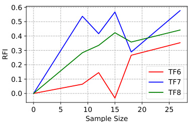
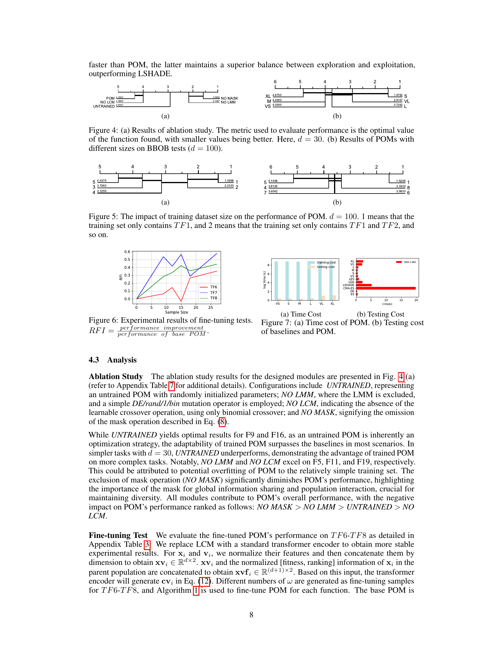
This figure shows the experimental results of fine-tuning tests on three composite functions (TF6-TF8) by using different numbers of samples. The RFI (Relative Performance Improvement) metric is used to evaluate the performance of the fine-tuned POM compared to the base POM. The x-axis represents the number of samples used for fine-tuning, while the y-axis shows the RFI for each function. The graph shows that as the number of samples used for fine-tuning increases, the performance of POM improves.

This figure shows the training and testing time costs of different optimization algorithms. The left panel (a) shows the training time cost of POM with different architecture settings (VS, S, M, L, VL, XL), demonstrating the training time increases with more complex architectures. The right panel (b) compares the testing time cost of POM against other baseline algorithms (LES, LGA, LSHADE, CMA-ES, DE, ES), highlighting POM’s superior efficiency in testing time.

This figure visualizes the LMM (Learned Mutation Module) strategy’s evolution across generations (steps 1, 50, and 100) for four different functions (F1-F4) from the BBOB benchmark. The heatmaps show the weights assigned by each individual in the population to others during the mutation process. Darker colors represent stronger weights, and blank cells represent masked elements.

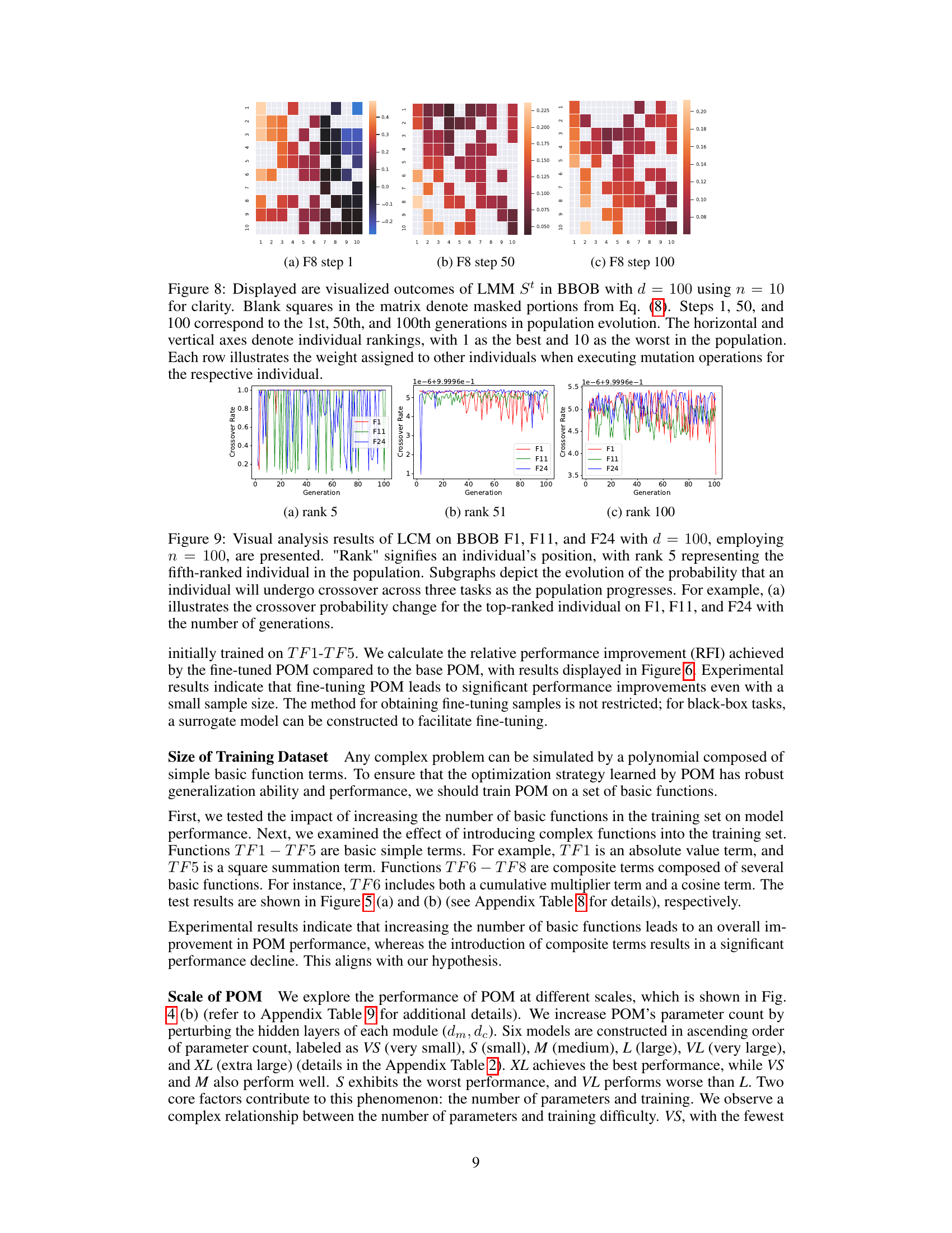
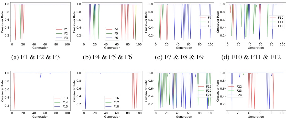
This figure presents a visual analysis of the LCM (Learned Crossover Module) performance on three different BBOB (Black-box Optimization Benchmark) functions (F1, F11, and F24) with dimension 100 and population size 100. It focuses on the crossover probability evolution for individuals ranked 5th in the population across generations. The subplots (a), (b), and (c) show the evolution of crossover probabilities for the top-ranked, 51st-ranked, and 100th-ranked individuals, respectively, across the three BBOB functions. This visualization helps understand how LCM adapts its crossover strategy across various tasks and individual rankings over generations.

This figure shows the results of a critical difference diagram comparing seven different black-box optimization algorithms across 24 benchmark problems in two different dimensions (30 and 100). The Wilcoxon-Holm statistical test was used to determine if there are statistically significant differences in the performance of the algorithms. Higher scores indicate that an algorithm consistently outperforms others. Horizontal lines connecting algorithms show that there is no statistically significant difference in performance between them.

This figure presents a critical difference diagram showing the performance comparison of seven different black-box optimization algorithms across 24 benchmark functions from the BBOB suite. The algorithms are compared in terms of their average performance across the 24 functions, with the x-axis representing the rank of the algorithm based on average performance. Algorithms grouped together by a horizontal line are not statistically significantly different in terms of performance. This type of diagram helps to visualize the relative ranking of different optimization algorithms. The dimension of the problem (number of variables to optimize) is 500.

This figure compares the performance of the Pretrained Optimization Model (POM) against several baseline algorithms on 24 benchmark functions from the BBOB suite. The x-axis represents the number of function evaluations, and the y-axis shows the log of the error (distance from the optimal solution). Each line represents a different algorithm, illustrating their convergence speed and effectiveness in finding optimal solutions. The shaded area shows the standard deviation of the POM’s performance across multiple runs.

This figure presents a comparison of the convergence speed of different optimization algorithms on 24 benchmark functions from the BBOB suite. Each subplot shows the log convergence curve (log of the function’s value over the number of iterations) for a specific function. The algorithms being compared are POM (the proposed algorithm), CMA-ES, DE, ES, LES, LGA, and L-SHADE. The figure visually demonstrates POM’s superior convergence performance on many of the benchmark functions compared to the other state-of-the-art methods.

This figure illustrates the architecture of the Pretrained Optimization Model (POM) and its training and testing processes. The architecture (a) shows three main components: LMM (Learning Mutation Module), LCM (Learning Crossover Module), and SM (Selection Module). The training process (b) shows how POM is trained using gradient-based methods on a set of differentiable training functions. The testing process (c) demonstrates how POM generalizes to unseen, potentially non-differentiable target tasks using only function evaluations, without any further training.
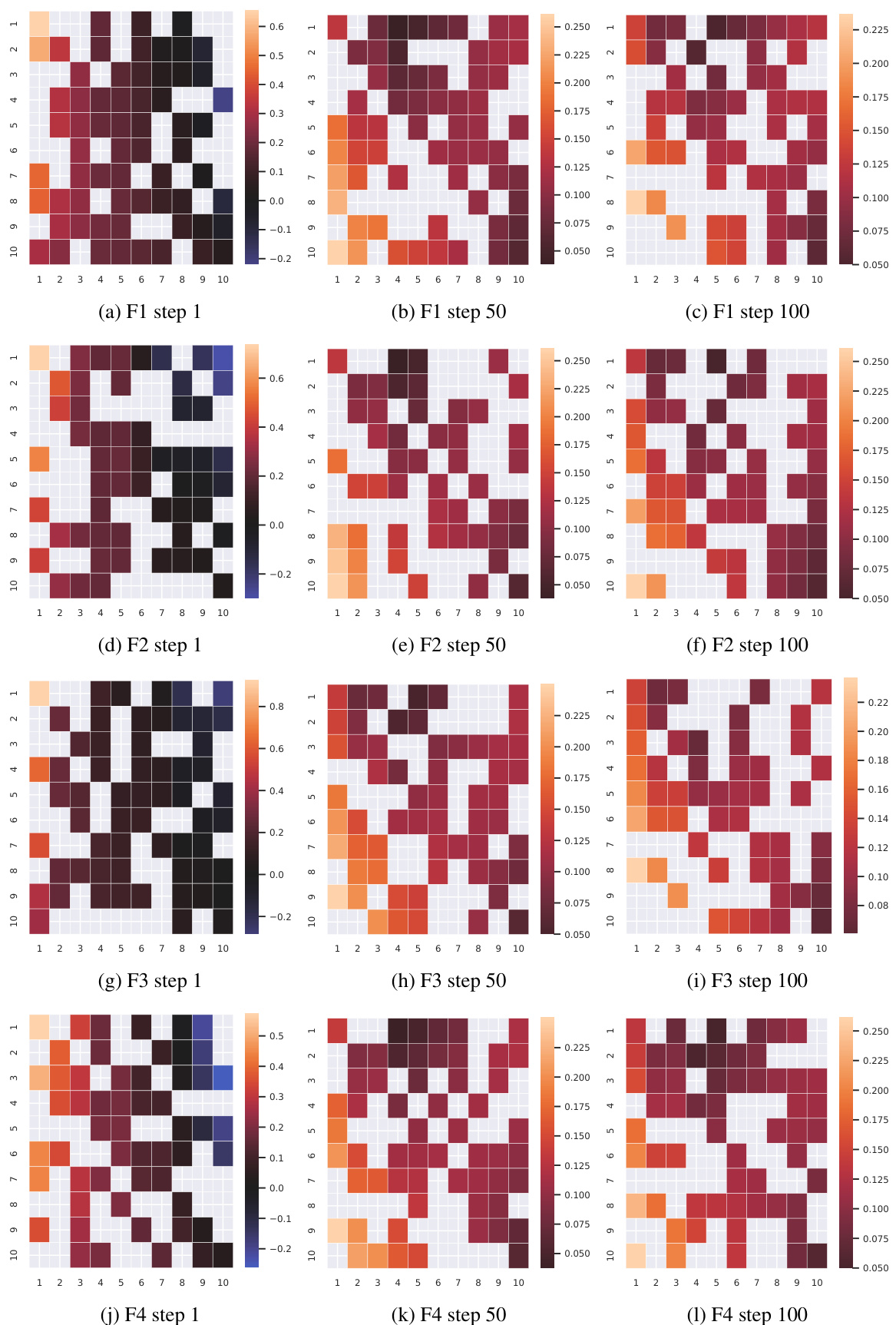
This figure visualizes the outcomes of the LMM (Learned Mutation Module) at different steps (1, 50, and 100) of the optimization process. It shows the weight assigned to other individuals when performing mutation operations for each individual, using a heatmap. Blank squares represent masked parts. The visualization helps understand how LMM dynamically generates mutation strategies across generations.

This figure illustrates the architecture of the Pretrained Optimization Model (POM), including its three main components: LMM, LCM, and SM. It also shows the training and testing processes for POM. The training process uses a differentiable training function to optimize the parameters of POM. The testing process applies the trained model to a target task, which may or may not be differentiable, to find the optimal solution without further parameter tuning.
This figure illustrates the architecture of the Pretrained Optimization Model (POM), a novel population-based optimizer for zero-shot black-box optimization. It shows the process of training POM on a differentiable training function set and then applying it to a new, potentially non-differentiable, task. The training phase uses an iterative process over T steps, leveraging information from the population of individuals (X) to learn a robust optimization strategy (θ). In the testing phase, the trained model is directly applied to solve a new target task, f, without gradient information. The figure highlights the three major components of POM: LMM, LCM, and SM, illustrating the model’s ability to generalize.

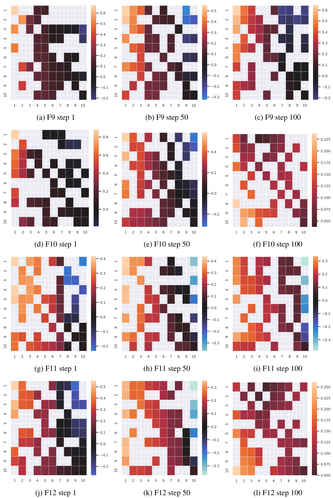
This figure visualizes the results of the mutation strategy (St) of the LMM module in POM on four different BBOB functions (F13 to F16). Each subfigure shows a heatmap representing the weight assigned to other individuals when performing mutation operations for the corresponding individual. The heatmaps are shown for three different generations (steps 1, 50, and 100), providing insights into how the strategy evolves over time. Darker colors indicate stronger weights. The rows represent the individual performing the mutation, and the columns represent the individuals influencing that mutation.

This figure visualizes the output of the LMM module (LMM) in the POM algorithm. The LMM module generates candidate solutions for each individual in a population. The visualization shows how the weights assigned to other individuals change across different generations (steps 1, 50, 100) for each individual in the population. Blank squares represent masked portions of the matrix, as per Equation (8).

This figure illustrates the architecture of the Pretrained Optimization Model (POM), its training process, and its testing process. The training process is gradient-based, while the testing process can be performed without gradient information. The overall architecture consists of three modules: LMM (Learned Mutation Module), LCM (Learned Crossover Module), and SM (Selection Module).

This figure illustrates the architecture of the Pretrained Optimization Model (POM), a novel population-based optimizer designed for zero-shot black-box optimization. It details three main components: LMM (Learned Mutation Module), LCM (Learned Crossover Module), and SM (Selection Module). The training process involves iteratively generating and updating the population based on a training function that must be differentiable. In contrast, the testing phase applies the trained model directly to a new objective task without requiring gradient information, enabling zero-shot optimization.

This figure compares the performance of the Pretrained Optimization Model (POM) against several other optimization algorithms on a set of 24 benchmark functions from the BBOB suite. The x-axis represents the number of generations (iterations) of the algorithm, and the y-axis represents the negative log of the error, showing the convergence speed and accuracy of each algorithm. Lower values indicate faster convergence and better performance. The figure visualizes the convergence speed and shows how POM outperforms state-of-the-art methods, especially for high-dimensional tasks. The figure is broken into subfigures, each showing the results for a subset of the benchmark functions.
This figure illustrates the overall architecture of the Pretrained Optimization Model (POM), including its three main components: LMM, LCM, and SM. It also shows the training and testing processes. The training process involves iteratively updating the POM parameters using a gradient-based optimizer on a set of training functions. The testing process involves directly applying the trained POM to a target task without fine-tuning or requiring gradient information.

This figure compares the performance of POM against other state-of-the-art black-box optimization algorithms across 24 different functions within the BBOB benchmark. The dimension of the optimization problems (d) is set to 30, and the results are presented as log convergence curves. Each curve depicts the performance of a specific algorithm over the course of 100 generations. This visualization allows for a direct comparison of convergence rates and effectiveness among the different methods.

This figure shows the architecture and the training and testing processes of the Pretrained Optimization Model (POM). Panel (a) details the components of POM, including the LMM, LCM, and SM modules, and how they process the initial random population to generate a final optimized population. Panel (b) illustrates the training loop, where POM is trained on a set of differentiable training functions to learn effective optimization strategies. The process involves iteratively updating the POM parameters based on the loss function until convergence. Panel (c) shows the testing phase, where the trained POM is directly applied to a new, potentially non-differentiable, target task to find the optimal solution without any further tuning.

This figure compares the convergence performance of POM against other baseline algorithms (CMA-ES, DE, ES, LES, LGA, LSHADE) across 24 functions from the BBOB benchmark. The x-axis represents the number of generations, and the y-axis represents the log of the function values. The plot shows how quickly each algorithm approaches the optimal solution (zero on the y-axis). The different lines represent the different algorithms, with POM generally converging faster than the baselines and exhibiting superior performance in high-dimensional tasks.
More on tables

This table lists the detailed parameter settings used for the different baseline algorithms compared in the paper’s experiments. It includes settings for CMA-ES, LSHADE, ES, DE, LGA, and LES, showing the specific values used for each algorithm’s hyperparameters. These parameters were either automatically adjusted, set to optimal values from previous literature, or tuned using a grid search. The table helps ensure reproducibility by clearly documenting the parameters used in each experiment.

This table shows the different hyperparameter settings used for the various model sizes of POM. It details the number of parameters, the dimension of the Multi-head Self-Attention (MSA) module’s input (dm), and the dimension of the Feedforward Network (FFN) module’s input (dc). These parameters are crucial for understanding the model’s complexity and performance across different scales.

This table lists eight additional training functions (TF1-TF8) used in the paper’s experiments. Each function includes a mathematical formula defining it, along with a specification of the range of its input variable ‘x’ and a parameter ‘ω’. These functions represent a diverse set of mathematical landscapes, designed to challenge and enhance the robustness of the POM algorithm during its training phase. The diversity in the functions’ characteristics, including modality (unimodal versus multimodal), separability, and the presence of asymmetry, helps to ensure that the trained POM model generalizes effectively to a wide variety of unseen optimization problems.
This table presents the results of the BBOB (Black-box Optimization Benchmark) experiments. POM (Pretrained Optimization Model) was trained using functions TF1-TF5 with a dimensionality (d) of 10. The table compares the performance of POM against several other optimization algorithms (ES, DE, CMA-ES, LSHADE, LES, and LGA) across 24 different BBOB test functions. The best performance for each function is highlighted in bold, and the near-best results are underlined. This allows for a direct comparison of POM’s performance on these standard benchmarks against state-of-the-art and classic algorithms.
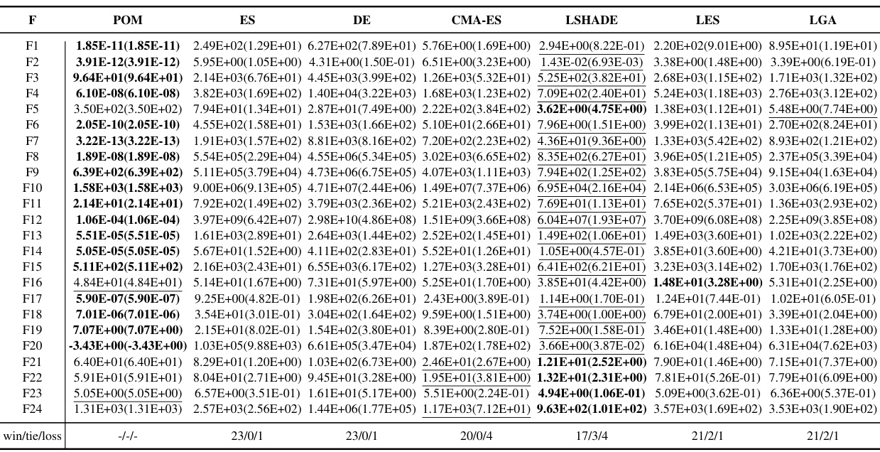
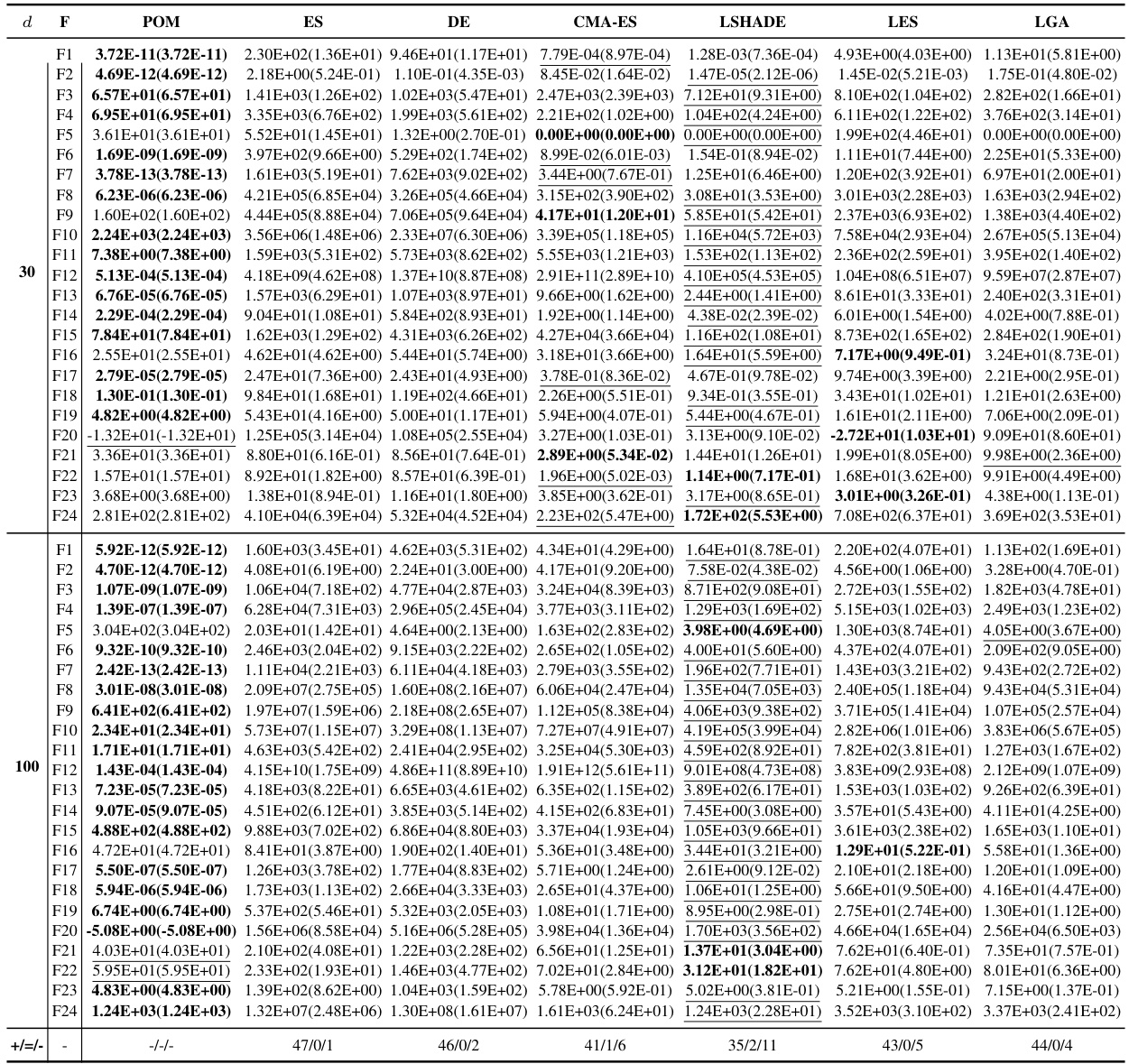
This table presents the results of additional experiments conducted on the BBOB benchmark with a dimensionality of 100. It compares the performance of POM against several other algorithms (ES, DE, CMA-ES, LSHADE, LES, and LGA) across 24 different functions (F1-F24). The best result for each function is highlighted in bold, and near-optimal results are underlined. This demonstrates the performance of POM in handling situations where the optimal solution of the function is slightly perturbed. The table provides a quantitative comparison to assess the algorithm’s robustness and generalisation ability.
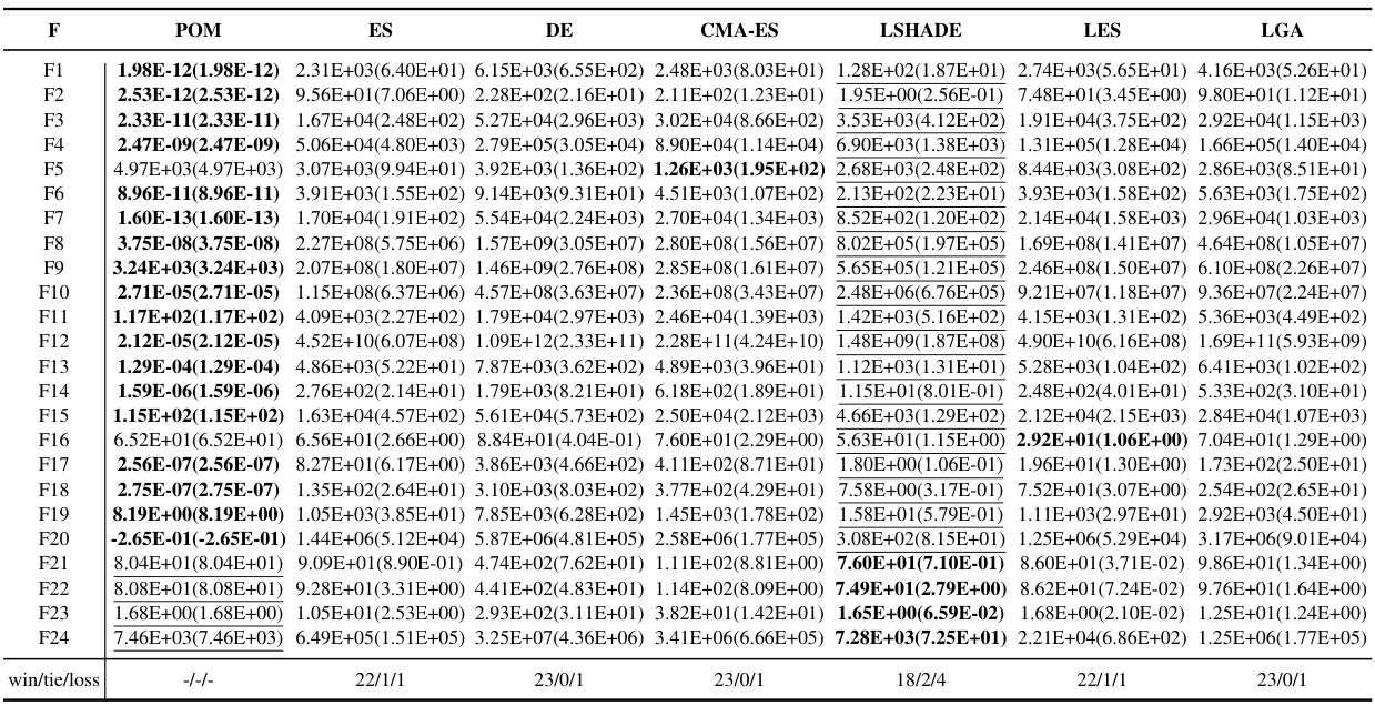
This table presents the results of additional experiments conducted on the BBOB benchmark with a dimensionality of 500. The table compares the performance of POM against several other algorithms (ES, DE, CMA-ES, LSHADE, LES, and LGA) across 24 different BBOB functions. The best result for each function is highlighted in bold, while suboptimal results are underlined. This data allows for a detailed comparison of POM’s performance relative to state-of-the-art methods in high-dimensional optimization problems.

This table presents the results of an ablation study conducted to evaluate the contribution of each module (LMM, LCM, SM, and Mask) in the POM architecture. The results show the optimal value (smaller is better) of the objective function achieved by POM and its variants on 24 benchmark functions from the BBOB suite. By removing one module at a time, the impact of each component on the overall performance is assessed, allowing for a quantitative analysis of their relative importance in the proposed optimization strategy.

This table presents the results of the proposed Pretrained Optimization Model (POM) on the Black-Box Optimization Benchmark (BBOB). POM was trained using functions TF1-TF5 with a dimension of 10 (d=10). The table shows the performance of POM across various BBOB functions (F1-F24), comparing it against other state-of-the-art algorithms. The best results for each function are highlighted in bold, and suboptimal results are underlined. This allows for a direct comparison of POM’s performance relative to existing methods for different BBOB functions.
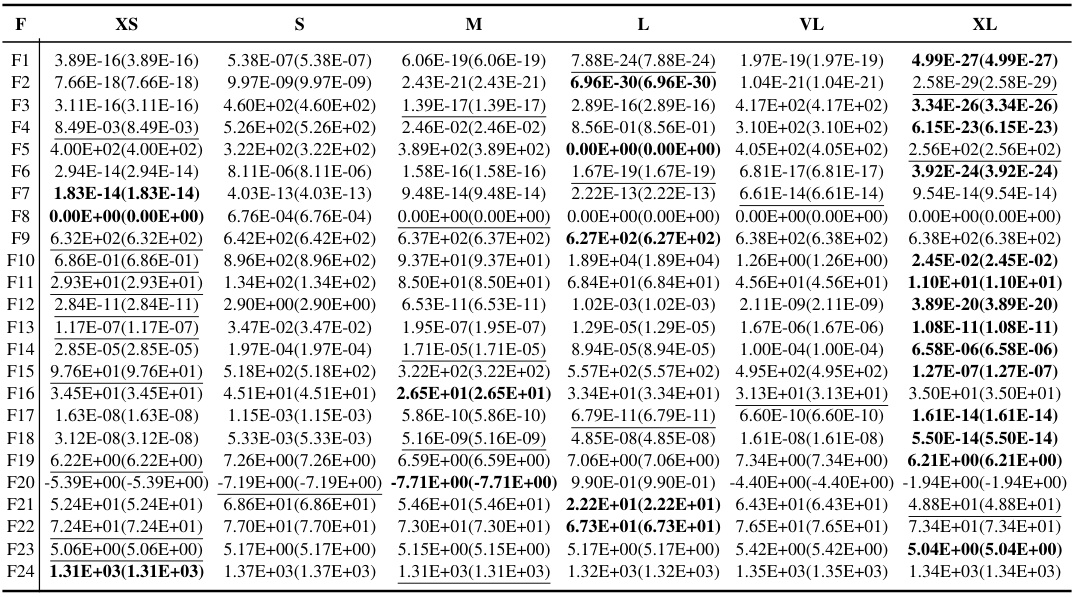
This table presents the results of POMs with different sizes (VS, S, M, L, VL, XL) tested on the BBOB benchmark functions with a dimensionality of 100. The best results for each function (F1-F24) are shown in bold, and the suboptimal results are underlined, allowing for a comparison of the algorithm’s performance at different scales. Each result represents the mean (mean) and standard deviation (std) of the optimal values achieved.
Full paper#
