TL;DR#
Molecular dynamics (MD) simulations are crucial for understanding complex systems but face challenges due to the complex energy landscapes and slow convergence of traditional optimization methods. Coarse-graining (CG) techniques simplify the system by reducing degrees of freedom but often lead to inaccuracies and require force-matching and back-mapping steps. This is particularly problematic in systems like proteins where interactions occur on multiple scales.
This paper introduces neural network reparametrization as a novel approach to molecular simulations. Unlike traditional CG, this method uses a neural network to represent the fine-grained system as a function of coarse-grained modes. The flexibility of this approach allows for adjusting the system’s complexity in order to simplify the optimization process, which can significantly improve efficiency and accuracy. The method also eliminates the need for force-matching, thereby enhancing the accuracy of energy minimization. Importantly, the proposed framework incorporates graph neural networks and physically meaningful ‘slow modes’, which are naturally arising from the structure of physical Hessians, further accelerating convergence and helping guide the optimization toward more stable configurations.
Key Takeaways#
Why does it matter?#
This paper is important because it offers a novel and efficient framework for molecular simulations, addressing challenges in traditional methods. It introduces neural network reparametrization, a flexible alternative to coarse-graining, improving optimization speed and accuracy. This opens new avenues for simulating complex molecular systems and can benefit researchers in various fields, including materials science, drug discovery, and protein engineering.
Visual Insights#

🔼 This figure provides a comprehensive overview of the neural reparametrization method proposed in the paper. It showcases three key aspects: different architectures for reparametrization (linear and GNN-based), a flowchart illustrating the step-by-step process of the method, and a detailed algorithmic description. The linear approach uses a straightforward linear projection of latent variables (Z) onto slow modes (Ψslow), while the GNN approach leverages the slow modes to construct a graph, then uses graph convolutional networks (GCNs) to perform reparametrization. The flowchart visually guides the reader through the key computational steps (Hessian computation, slow mode extraction, GNN-based reparametrization, and optimization), enhancing understanding. The detailed algorithm provides a precise, code-like description of the procedure.
read the caption
Figure 1: Overview of the neural reparametrization method. Top: Architectures used for reparametrization. In linear reparametrization, X = ZTΨslow. In the GNN case, we use the slow modes to construct a graph with adjacency A = ΨslowΨslowT and use it in GCN layers to obtain X = gnn(Z). Left: Flowchart showing the key steps of the method. Right: Detailed algorithm for implementation.
In-depth insights#
Neural CG Approach#
A neural coarse-graining (CG) approach offers a novel way to accelerate molecular simulations. Unlike traditional CG methods that reduce the degrees of freedom, a neural network reparametrizes the system, flexibly adjusting the model’s complexity. This allows for continuous access to fine-grained details while potentially simplifying the optimization process, eliminating the need for force-matching. The use of graph neural networks (GNNs), informed by slow modes, significantly accelerates convergence. GNNs can incorporate CG modes as needed, offering a robust and efficient framework to handle complex energy landscapes. This method demonstrates significant advantages in both accuracy and speed, outperforming traditional optimization methods in challenging scenarios, such as protein folding with weak molecular forces.
GNN-based CG#
The proposed GNN-based coarse-graining (CG) method presents a significant advancement in molecular simulations. Unlike traditional CG methods that drastically reduce degrees of freedom, this approach uses neural networks to flexibly adjust the complexity of the system, sometimes even increasing it to simplify optimization. This overparametrization allows the model to dynamically represent fine-grained details, enhancing both efficiency and accuracy. A key innovation is the incorporation of graph neural networks (GNNs) informed by ‘slow modes’, which are inherently stable collective modes identified through spectral analysis. By focusing on these slow modes, the GNN method accelerates convergence to the global energy minima and consistently outperforms traditional optimization methods. The ability to seamlessly integrate arbitrary neural networks such as GNNs into the reparametrization framework offers great versatility. The elimination of force-matching and back-mapping procedures further simplifies the workflow and enhances scalability. Overall, this novel approach demonstrates substantial progress in molecular simulation by efficiently optimizing energy minimization and convergence speeds, opening pathways to simulate complex molecular systems more effectively.
Hessian Slow Modes#
The concept of “Hessian slow modes” centers on the observation that in molecular dynamics simulations, the optimization process is significantly hindered by the disparity in the rates at which different modes of the system evolve. Hessian eigenvalues, which determine these rates, reveal that some modes (slow modes) change incredibly slowly, causing convergence bottlenecks. These slow modes are closely related to the inherent symmetries and structure of the potential energy functions describing molecular interactions. Identifying and utilizing these slow modes becomes crucial for efficient optimization. The research cleverly leverages this insight by incorporating slow modes within a neural network framework to cleverly guide the system towards lower energy configurations, improving both accuracy and speed. This approach represents a significant departure from traditional coarse-graining methods that focus solely on reducing the degrees of freedom, offering a more flexible, adaptive, and efficient strategy for molecular simulations.
Protein Folding Tests#
Protein folding, a complex process, is computationally expensive to simulate accurately. This research uses neural network reparametrization to accelerate energy minimization and convergence, offering a novel approach to traditional coarse-graining methods. The core innovation lies in the flexible adjustment of system complexity; it is not strictly limited to reducing degrees of freedom, sometimes increasing it to simplify optimization. This is particularly advantageous when dealing with complex energy landscapes characterized by numerous local minima and saddle points, as in protein folding. The approach enhances both efficiency and accuracy by avoiding force-matching and providing continuous access to fine-grained modes. The use of Graph Neural Networks (GNNs) offers further advantages, incorporating slow modes to guide the optimization effectively and consistently outperforming traditional methods. Experiments on synthetic and real protein structures show significant advancements in both accuracy and speed of convergence to the deepest energy states, highlighting the efficacy of this novel framework for simulating complex molecular systems. The data-free nature of the optimization method is another key strength, eliminating reliance on extensive training datasets and making it widely applicable.
Future Directions#
Future research could explore extending the neural network reparametrization approach to handle more complex molecular systems and diverse force fields. Improving the efficiency of the GNN architecture is crucial for scaling to larger systems and longer simulations. Investigating alternative neural network architectures beyond GNNs, such as transformers or other advanced deep learning models, could potentially enhance performance and flexibility. A particularly exciting area would be developing methods to automatically identify relevant slow modes without requiring spectral analysis, improving the robustness and general applicability of the approach. Further work should also focus on incorporating more sophisticated physical knowledge into the framework to guide the optimization process. Finally, the application of this framework to other challenging scientific simulations beyond molecular dynamics, such as materials science or fluid dynamics, should be investigated.
More visual insights#
More on figures

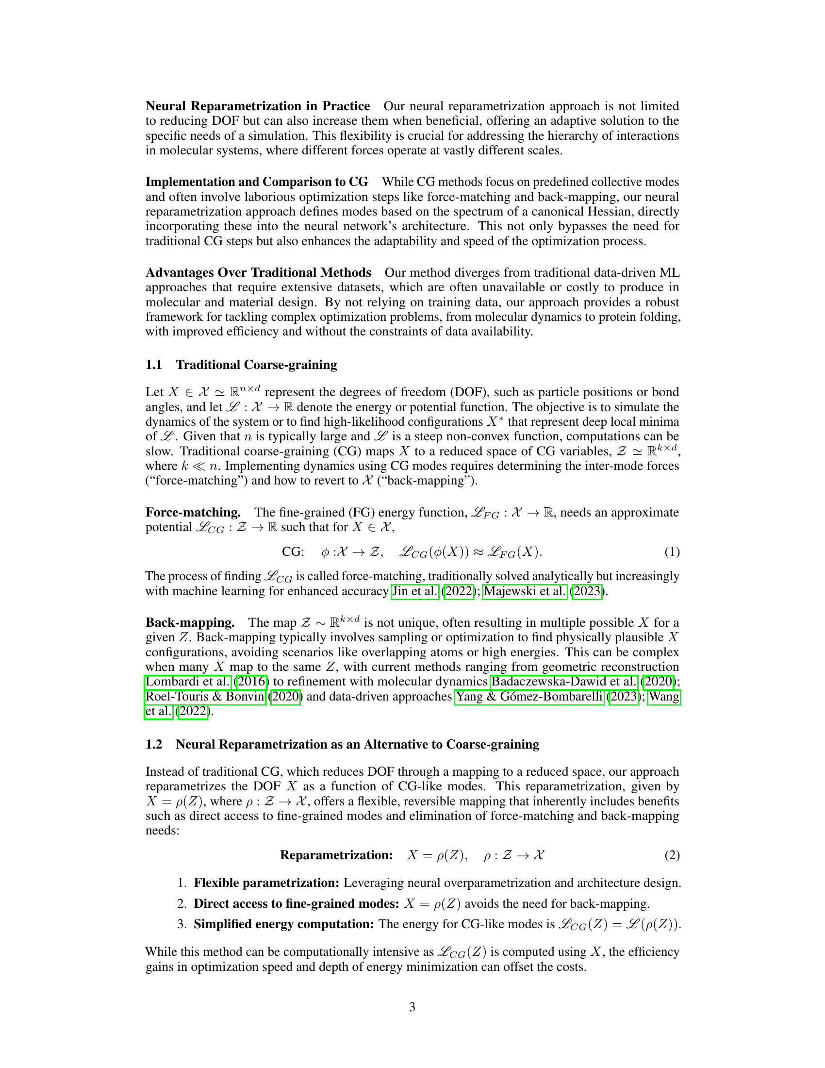
🔼 This figure shows the results of synthetic loop experiments using three different methods: Gradient Descent (GD), Coarse-graining with Reparametrization (CG Rep), and Graph Neural Network (GNN). Two scenarios are compared: one with both bond and Lennard-Jones (LJ) potentials (Bond+LJ), and one with only LJ potentials (Pure LJ). The GNN method consistently outperforms the others, especially in the more challenging Pure LJ scenario, where it is the only method that successfully forms the loop structure.
read the caption
Figure 2: Synthetic loop experiments. Example runs of the synthetic loop experiments with n = 400 nodes. On the left (Bond+LJ), the potential is the sum of a quadratic bond potential Ebond and a weak LJ (12,6) ELJ. The bonds form a line graph Abond connecting node i to i + 1, and a 10 weaker Aloop connecting node i to i + 10 via the LJ potential. To the right (Pure LJ) where the interactions are all LJ, but with a coupling matrix A = Abond + 0.1Aloop. In Bond+LJ, GD already finds good energies and the configuration is reasonably close to a loop, though flattened. Both linear CG reparametrization (CG Rep) and GNN also find a good layout. The pure LJ case is much more tricky. But in most runs, GD almost gets the layout, but some nodes remain far away. The CG Rep fails to bring all the pieces together. Only GNN succeeds in finding the correct layout.

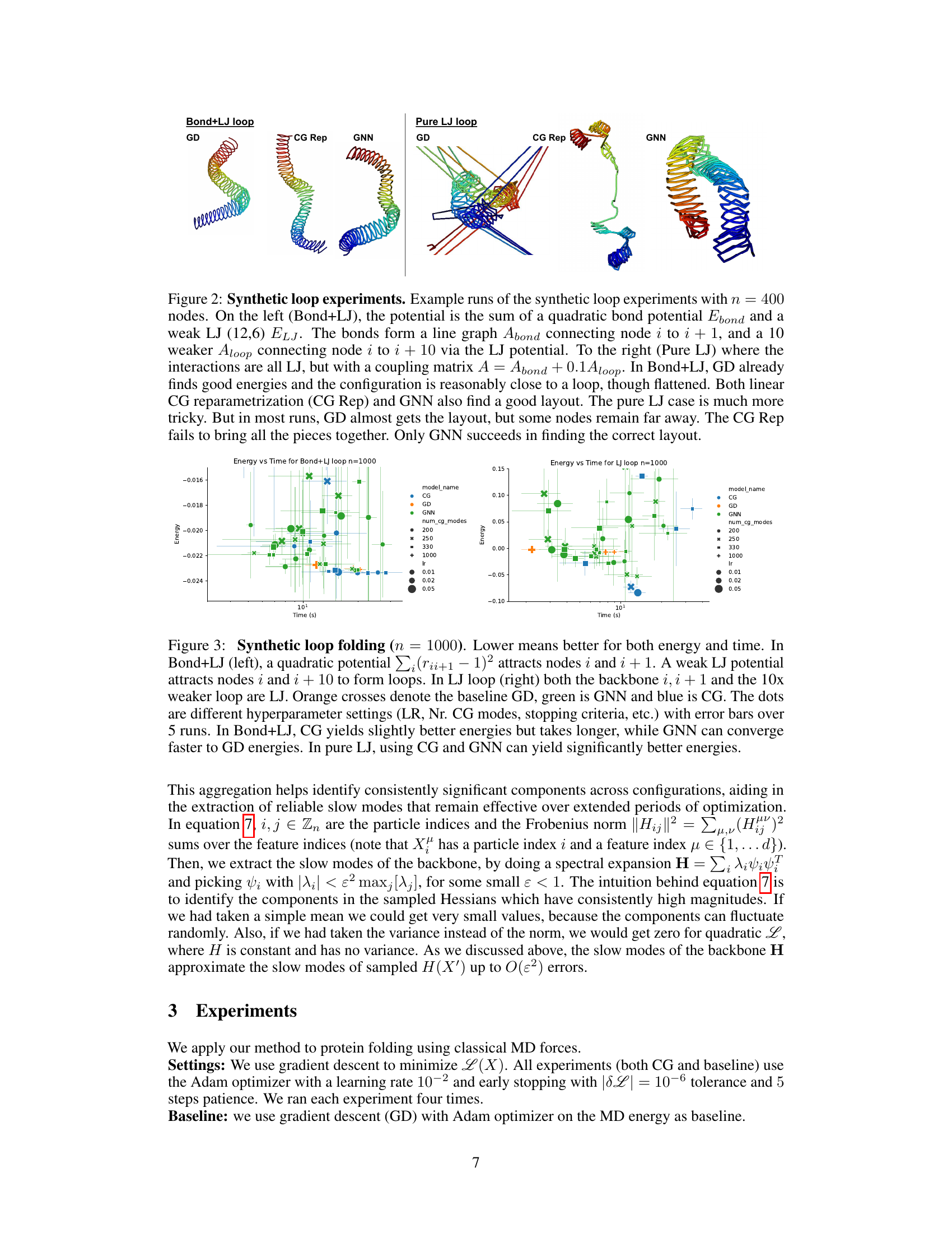
🔼 This figure compares the performance of three methods (Gradient Descent, Coarse-Graining, and Graph Neural Network) on two synthetic loop folding tasks with 1000 nodes. The left panel shows results for a system with both bond and Lennard-Jones (LJ) potentials, while the right shows results for a system with only LJ potentials. The plots show energy achieved versus time taken. The results demonstrate that the GNN method outperforms the other two, particularly in the challenging all-LJ system, achieving better energy and faster convergence.
read the caption
Figure 3: Synthetic loop folding (n = 1000). Lower means better for both energy and time. In Bond+LJ (left), a quadratic potential ∑i (rii+1 – 1)² attracts nodes i and i + 1. A weak LJ potential attracts nodes i and i + 10 to form loops. In LJ loop (right) both the backbone i, i + 1 and the 10x weaker loop are LJ. Orange crosses denote the baseline GD, green is GNN and blue is CG. The dots are different hyperparameter settings (LR, Nr. CG modes, stopping criteria, etc.) with error bars over 5 runs. In Bond+LJ, CG yields slightly better energies but takes longer, while GNN can converge faster to GD energies. In pure LJ, using CG and GNN can yield significantly better energies.

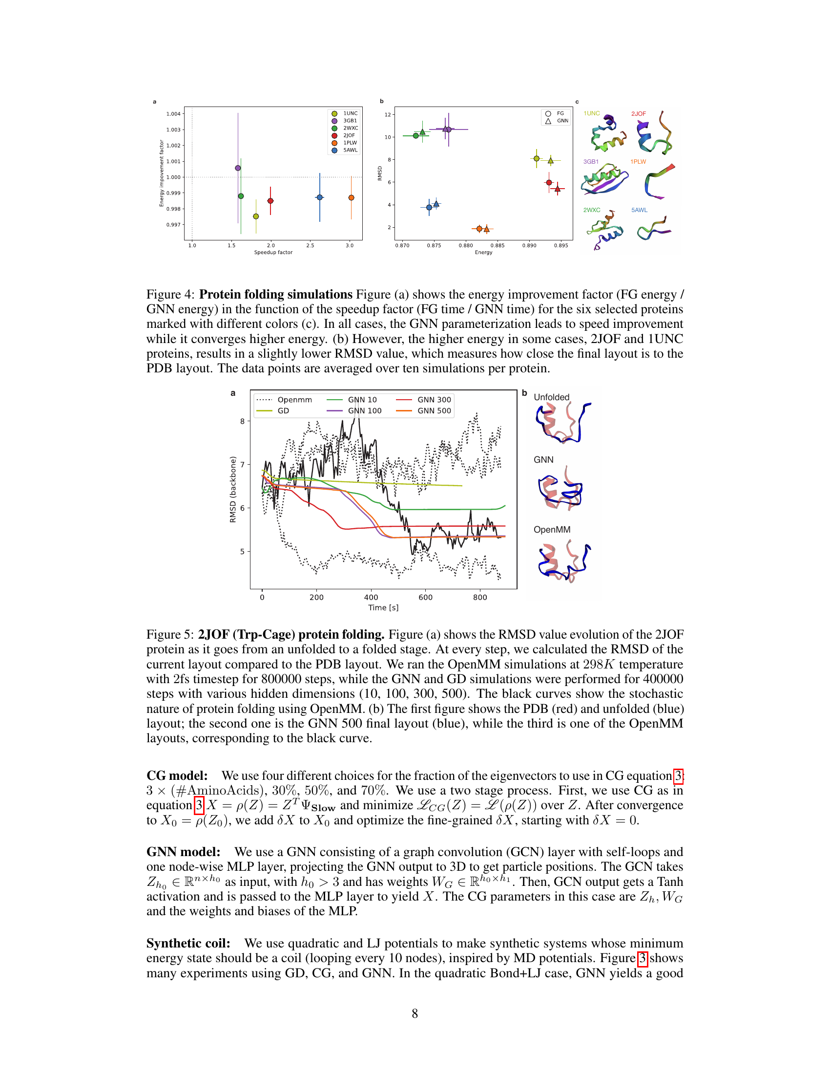
🔼 The figure shows the results of protein folding simulations using three different methods: fine-grained (FG), gradient descent (GD), and graph neural network (GNN). Panel (a) compares the energy improvement factor (ratio of FG energy to GNN energy) to the speedup factor (ratio of FG time to GNN time) across six different proteins. The GNN consistently shows improvement in speed while having slightly higher energy in some cases, as shown in panel (b). Panel (b) shows that this slightly higher energy does not always correspond to a higher root mean square deviation (RMSD), which indicates that the GNN structures are still quite close to the correct structures. Panel (c) shows the final structures for each of the six proteins obtained with the three methods, confirming that GNN is able to produce accurate predictions.
read the caption
Figure 4: Protein folding simulations Figure (a) shows the energy improvement factor (FG energy / GNN energy) in the function of the speedup factor (FG time / GNN time) for the six selected proteins marked with different colors (c). In all cases, the GNN parameterization leads to speed improvement while it converges higher energy. (b) However, the higher energy in some cases, 2JOF and 1UNC proteins, results in a slightly lower RMSD value, which measures how close the final layout is to the PDB layout. The data points are averaged over ten simulations per protein.
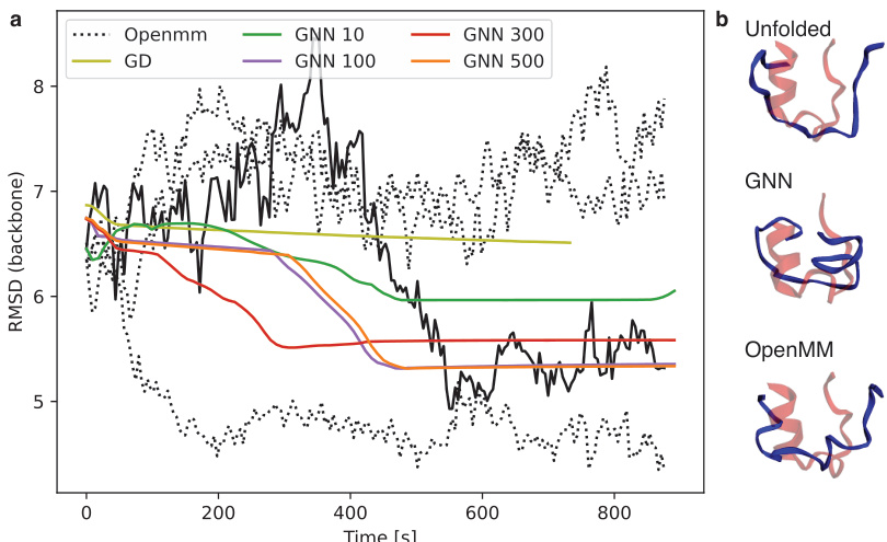
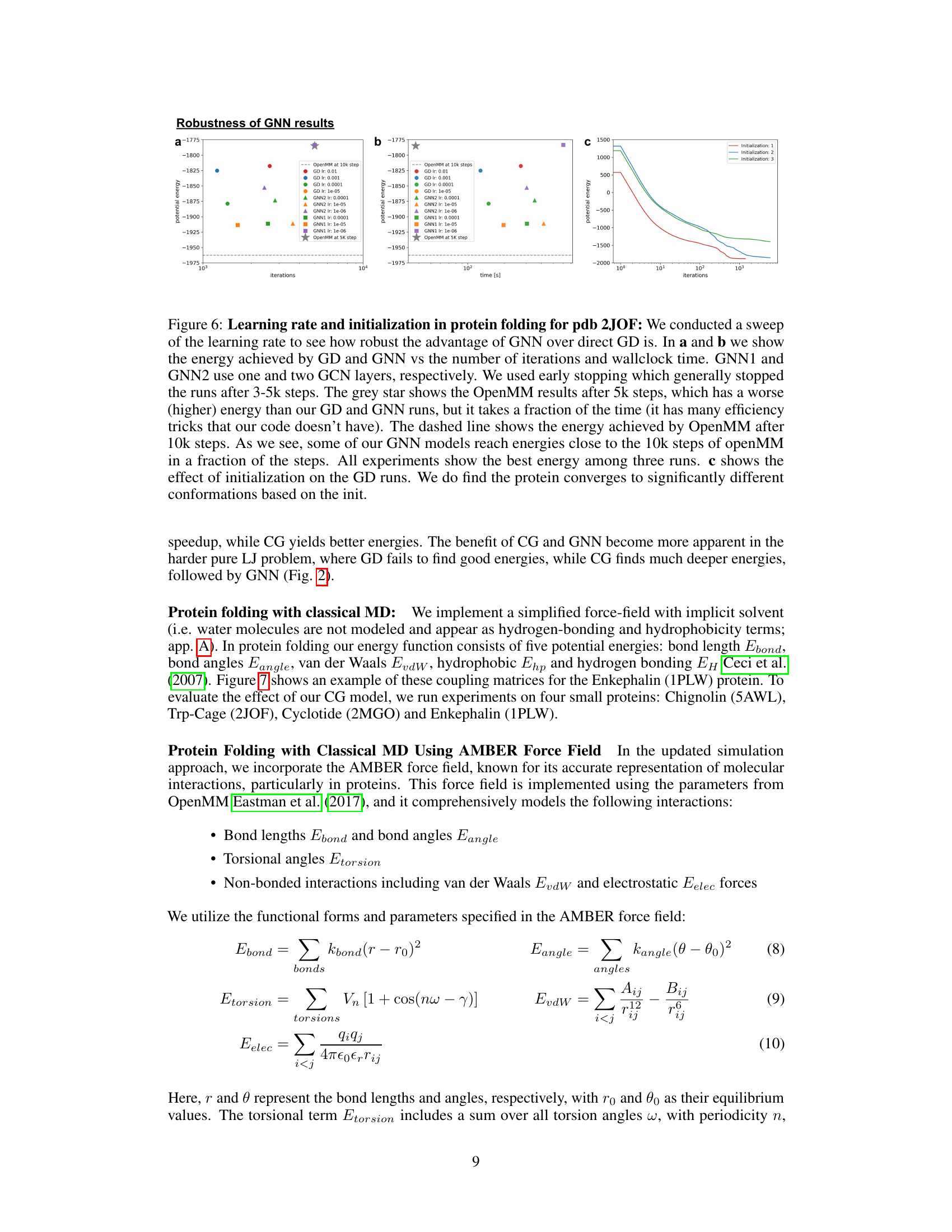
🔼 This figure shows the results of protein folding simulations for the Trp-Cage protein (2JOF). Panel (a) presents a graph comparing the root-mean-square deviation (RMSD) from the known folded structure over time for different methods: OpenMM, gradient descent (GD), and graph neural networks (GNN) with varying numbers of hidden units. The plot illustrates the convergence of the different methods towards the folded state, highlighting the faster convergence and lower RMSD achieved by GNN with more hidden units compared to OpenMM and GD. The stochastic nature of protein folding using OpenMM is also demonstrated. Panel (b) shows 3D visualizations of the protein in unfolded, GNN-optimized, and OpenMM-optimized states, offering a visual comparison of the conformations.
read the caption
Figure 5: 2JOF (Trp-Cage) protein folding. Figure (a) shows the RMSD value evolution of the 2JOF protein as it goes from an unfolded to a folded stage. At every step, we calculated the RMSD of the current layout compared to the PDB layout. We ran the OpenMM simulations at 298K temperature with 2fs timestep for 800000 steps, while the GNN and GD simulations were performed for 400000 steps with various hidden dimensions (10, 100, 300, 500). The black curves show the stochastic nature of protein folding using OpenMM. (b) The first figure shows the PDB (red) and unfolded (blue) layout; the second one is the GNN 500 final layout (blue), while the third is one of the OpenMM layouts, corresponding to the black curve.

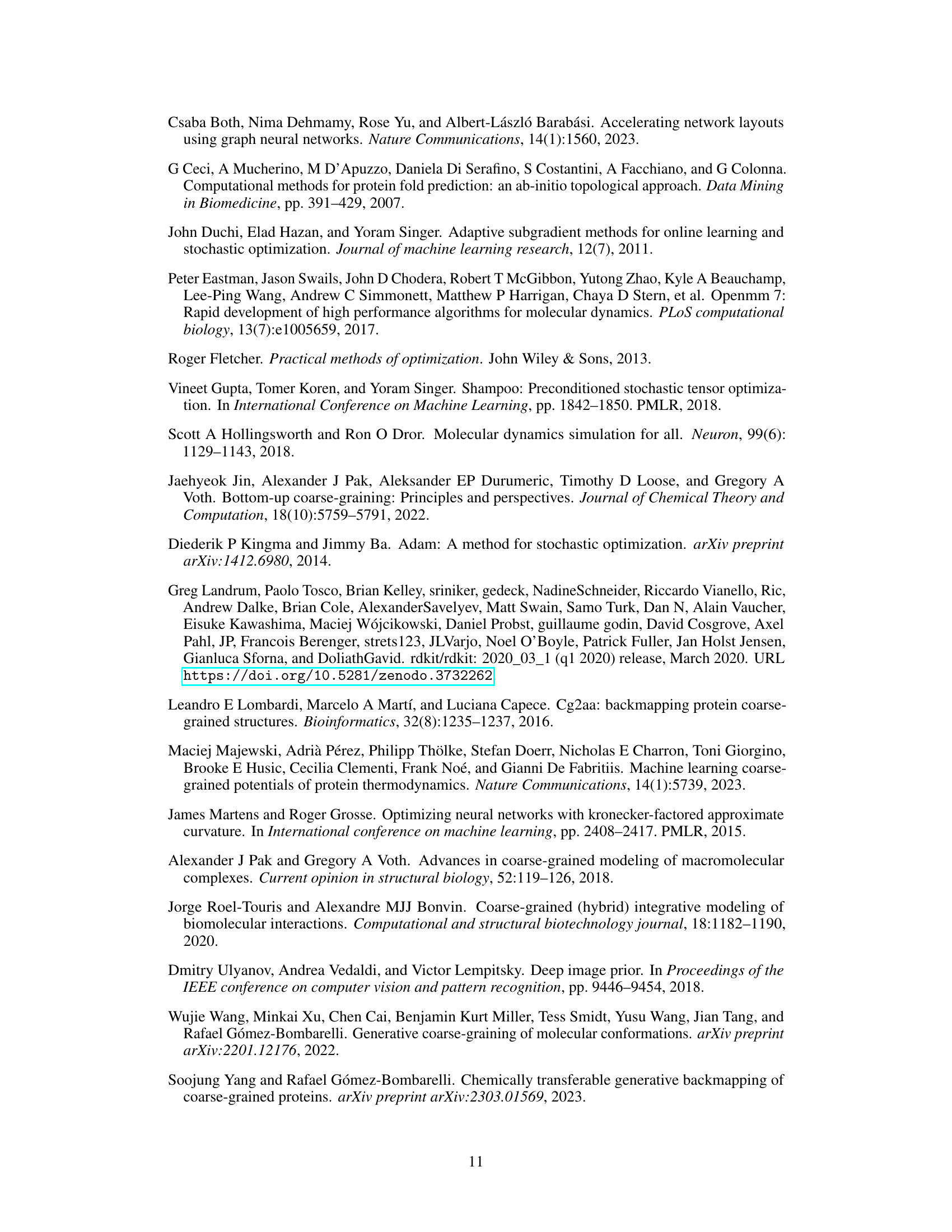
🔼 The figure shows the results of experiments on the robustness of the GNN model in protein folding. Subfigure (a) and (b) compare the potential energy achieved by gradient descent (GD) and the GNN model with varying learning rates and against OpenMM, demonstrating the GNN’s faster convergence to lower energies. Subfigure (c) shows the impact of different initializations on GD convergence, indicating sensitivity to initial conditions. The results highlight the GNN’s advantages in terms of energy minimization and convergence speed.
read the caption
Figure 6: Learning rate and initialization in protein folding for pdb 2JOF: We conducted a sweep of the learning rate to see how robust the advantage of GNN over direct GD is. In a and b we show the energy achieved by GD and GNN vs the number of iterations and wallclock time. GNN1 and GNN2 use one and two GCN layers, respectively. We used early stopping which generally stopped the runs after 3-5k steps. The grey star shows the OpenMM results after 5k steps, which has a worse (higher) energy than our GD and GNN runs, but it takes a fraction of the time (it has many efficiency tricks that our code doesn't have). The dashed line shows the energy achieved by OpenMM after 10k steps. As we see, some of our GNN models reach energies close to the 10k steps of openMM in a fraction of the steps. All experiments show the best energy among three runs. c shows the effect of initialization on the GD runs. We do find the protein converges to significantly different conformations based on the init.

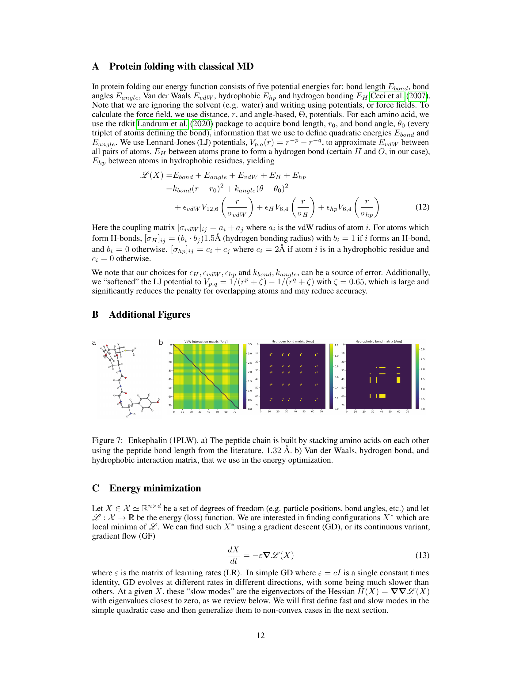
🔼 This figure shows the structure of the Enkephalin (1PLW) peptide and its interaction matrices. Panel (a) presents the 3D structure of the peptide chain, where amino acids are stacked using a bond length of 1.32 Å. Panels (b) display the interaction matrices used in the energy optimization, including Van der Waals (VdW), hydrogen bond, and hydrophobic bond interactions. These matrices visually represent the strengths of interactions between pairs of atoms in the peptide.
read the caption
Figure 7: Enkephalin (1PLW). a) The peptide chain is built by stacking amino acids on each other using the peptide bond length from the literature, 1.32 Å. b) Van der Waals, hydrogen bond, and hydrophobic interaction matrix, that we use in the energy optimization.
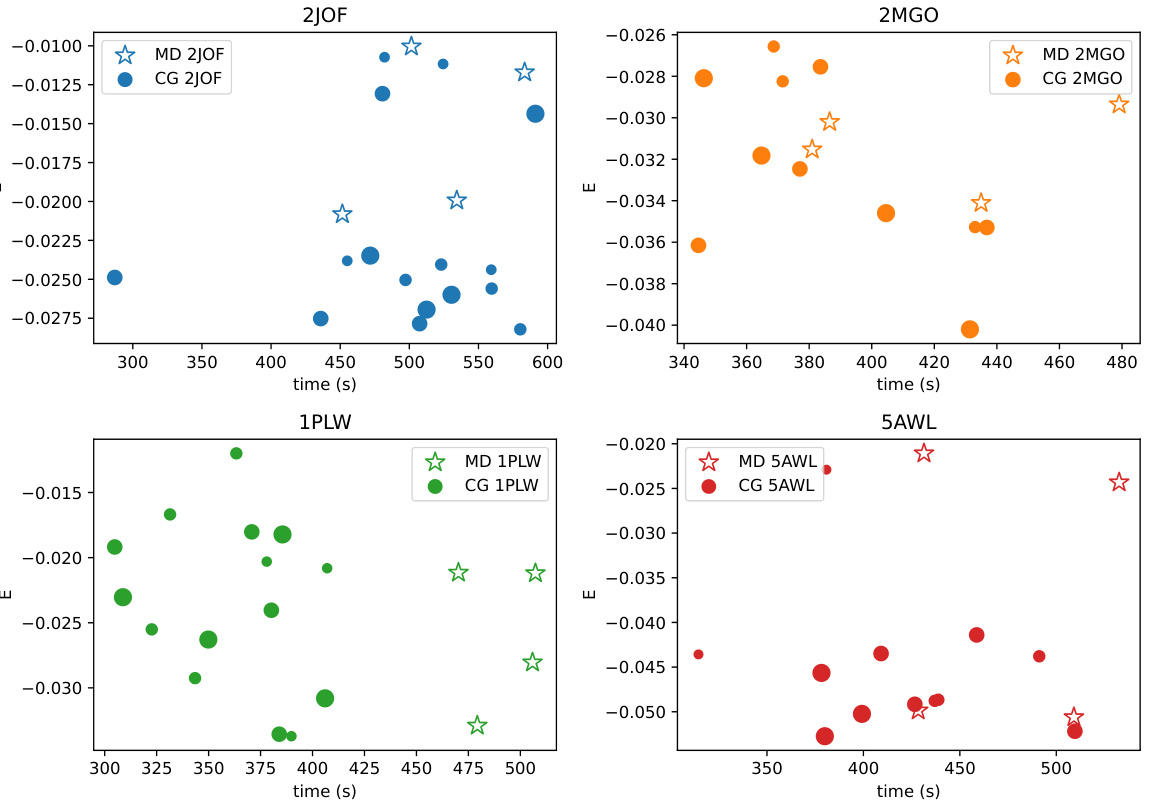
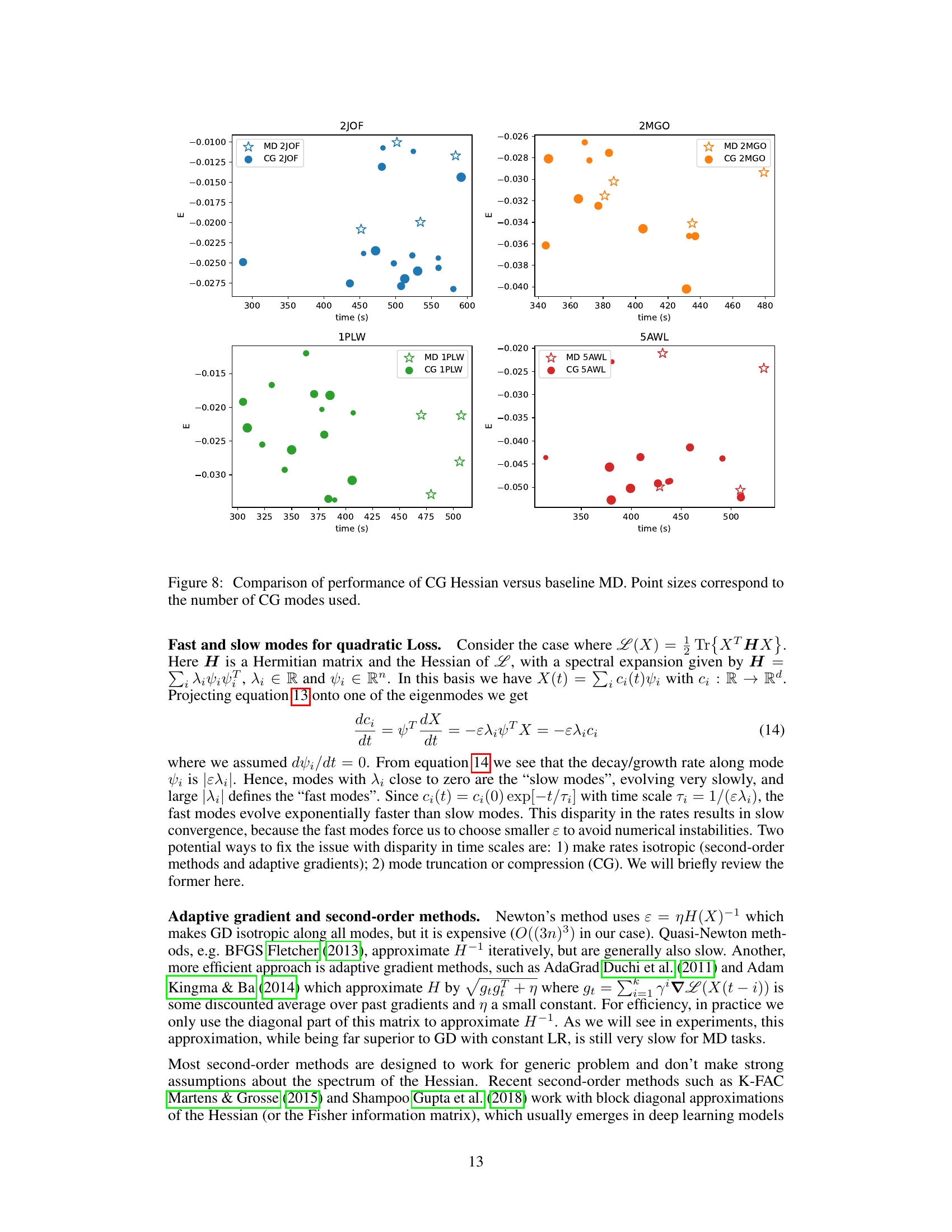
🔼 This figure compares the performance of the coarse-graining (CG) method using the Hessian with the baseline molecular dynamics (MD) method. The x-axis represents the time taken for the simulation to complete, and the y-axis represents the energy reached. Different colors represent simulations for different proteins (2JOF, 2MGO, 1PLW, 5AWL). Each point shows a single simulation run and its size indicates the number of collective modes used in the CG method. The figure demonstrates that the CG method is able to reach lower energy states in a similar amount of time as compared to the baseline MD method, suggesting that CG is an effective way to accelerate molecular dynamics simulations.
read the caption
Figure 8: Comparison of performance of CG Hessian versus baseline MD. Point sizes correspond to the number of CG modes used.

🔼 This figure compares the final folded structures of the 2JOF protein obtained using different methods: standard molecular dynamics (MD) and coarse-graining (CG) with varying numbers of eigenvectors. The dashed boxes highlight the minimum energy conformation for each method, while the solid box highlights the absolute minimum energy conformation. It illustrates the effectiveness of the CG method in achieving a structure closer to the true minimum energy conformation, showcasing the impact of the number of eigenvectors used.
read the caption
Figure 9: The folded structures of the 2JOF protein by using the CG and baseline method. The numbers in front of the rows are the numbers of eigenvectors used in the CG reparametrization. Dashed frames show the minimum energy embedding in each case, while the thick line frame highlights the absolute minimum layout.
Full paper#
