TL;DR#
Physics-Informed Neural Networks (PINNs) are a powerful tool for solving partial differential equations (PDEs), but their training dynamics are poorly understood, especially for nonlinear PDEs. Existing theoretical analyses often rely on the Neural Tangent Kernel (NTK) framework, which assumes an overparameterized network and simplifies the training process. However, this simplification breaks down for nonlinear PDEs, where the NTK’s properties change significantly during training. This leads to issues like slow convergence and spectral bias, hindering the performance of PINNs.
This research delves into the theoretical differences between training PINNs for linear versus nonlinear PDEs. The authors demonstrate that the NTK framework is inadequate for nonlinear PDEs due to the stochastic nature of the kernel at initialization, its dynamic behavior during training, and the non-vanishing Hessian. To overcome these limitations, they propose and thoroughly analyze using second-order optimization methods. Their theoretical results, backed by numerical experiments on various linear and nonlinear PDEs, show substantial performance improvements over first-order methods, particularly in terms of convergence speed and accuracy.
Key Takeaways#
Why does it matter?#
This paper is crucial for researchers using Physics-Informed Neural Networks (PINNs) as it reveals limitations of existing theoretical frameworks for nonlinear PDEs and proposes the use of second-order optimization methods for improved accuracy and speed. It challenges conventional wisdom, highlighting the need for new analytical tools and methodologies in this active field of research, opening avenues for future improvements in PINN training.
Visual Insights#

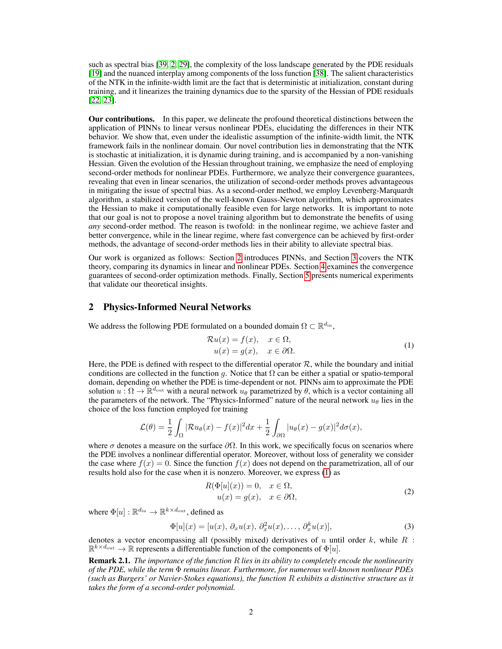
🔼 This figure shows the results of numerical experiments that validate the theoretical findings about the Neural Tangent Kernel (NTK) for Physics-Informed Neural Networks (PINNs). Part (a) compares the spectral norm of the NTK at initialization (K(0)) for linear and nonlinear partial differential equations (PDEs) as a function of the number of neurons (m). It demonstrates that, unlike the linear case, the NTK for nonlinear PDEs is not deterministic at initialization and its spectral norm shows high variability. Part (b) shows the evolution of the NTK during training (ΔK(t) = ||K(t) - K(0)||) for both linear and nonlinear PDEs. The results confirm that the NTK for nonlinear PDEs is not constant during training, unlike the linear case.
read the caption
Figure 1: (a) Mean and standard deviation of the spectral norm of K(0) as a function of the number of neurons m for 10 independent experiments. Left: linear case. Right: nonlinear case. (b) Mean and standard deviation of ΔK(t) := ||K(t) - K(0)|| over the network’s width m, for 10 independent experiments. Left: linear case. Right: nonlinear case.

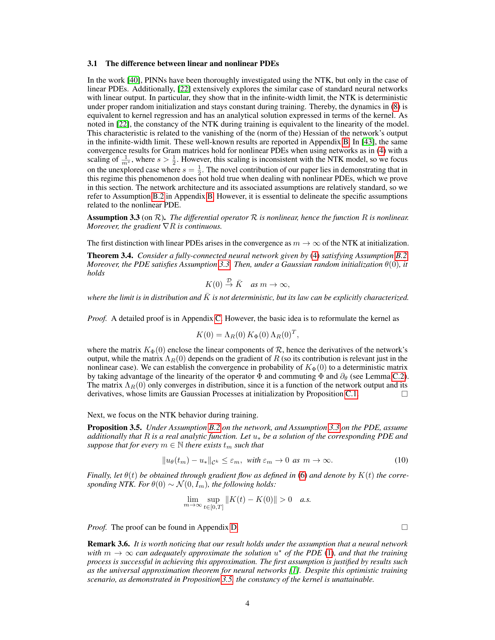
🔼 The table summarizes the key theoretical differences between applying PINNs to linear and nonlinear PDEs, focusing on the behavior of the Neural Tangent Kernel (NTK) and the Hessian matrix. It highlights that for linear PDEs, the NTK is deterministic and constant during training, with a sparse Hessian, leading to convergence bounds related to the minimum eigenvalue of the NTK. In contrast, for nonlinear PDEs, the NTK is random at initialization and dynamic during training, having a non-sparse Hessian, affecting convergence bounds which become related to the minimum eigenvalue of the time-dependent NTK or are 0 or 1 in the second-order case.
read the caption
Table 1: Comparison of the theoretical results for linear and nonlinear PDEs.
In-depth insights#
Nonlinear PINN Limits#
The limitations of Physics-Informed Neural Networks (PINNs) in the nonlinear regime are significant. The Neural Tangent Kernel (NTK) framework, commonly used to analyze PINN training dynamics, is shown to be inadequate for nonlinear Partial Differential Equations (PDEs). Unlike the linear case, the NTK is not deterministic and constant during training; instead, it’s stochastic at initialization and dynamic throughout training. Furthermore, the Hessian of the loss function does not vanish, even in the infinite-width limit, preventing the simplification afforded in the linear case. This necessitates the use of second-order optimization methods, such as Levenberg-Marquardt, to mitigate spectral bias and achieve faster convergence. Although second-order methods are shown to improve training and alleviate some challenges, their scalability remains a key limitation, requiring further investigation into efficient solutions for handling large-scale problems. The theoretical analysis is supported by numerical experiments across various PDEs, demonstrating the significant gap in behavior between the linear and nonlinear domains. This underscores the need for specialized techniques and tailored methods to effectively train PINNs for nonlinear systems.
NTK Dynamics Shift#
The Neural Tangent Kernel (NTK) is a powerful tool for analyzing the training dynamics of neural networks, particularly in the context of Physics-Informed Neural Networks (PINNs). A shift in NTK dynamics occurs when transitioning from linear to nonlinear partial differential equations (PDEs). In the linear regime, the NTK is deterministic and constant during training, simplifying analysis. However, for nonlinear PDEs, this assumption breaks down. The NTK becomes stochastic at initialization and dynamic throughout training, significantly complicating theoretical analysis and impacting the convergence behavior. This shift necessitates a reevaluation of traditional NTK-based analysis techniques and suggests that second-order optimization methods, which account for the non-vanishing Hessian, are superior for training PINNs solving nonlinear PDEs. This change also highlights the limitations of the infinite-width assumption frequently used in NTK analysis, emphasizing the need for further research considering finite-width networks and the impact of the Hessian on convergence guarantees.
Second-Order Edge#
The concept of a “Second-Order Edge” in a research paper likely refers to a sophisticated approach that goes beyond standard first-order methods for edge detection or analysis. This could involve analyzing curvature, gradients of gradients, or other higher-order differential properties to achieve superior edge detection accuracy and robustness. A second-order approach might be particularly useful for identifying subtle edges that are blurred or weakly defined, or for discriminating between true edges and noise. It might also lead to more accurate edge representation and analysis, providing information about edge sharpness and orientation that would not be available with first-order methods. Computational cost and complexity would likely be significantly higher, however, making real-time processing challenging. A key aspect of analyzing “Second-Order Edges” would likely focus on the development and evaluation of efficient algorithms, potentially leveraging parallel processing or specialized hardware. The paper would need to carefully compare and contrast its performance against existing first-order techniques, showcasing the advantages in specific applications, such as medical imaging, computer vision, or high-resolution microscopy.
Spectral Bias Fix#
Addressing spectral bias in Physics-Informed Neural Networks (PINNs) is crucial for improved accuracy and faster convergence, especially when dealing with high-frequency components in the solutions of Partial Differential Equations (PDEs). Spectral bias arises from the rapid decay of the Neural Tangent Kernel (NTK) eigenvalues, hindering the efficient learning of high-frequency details. This paper explores second-order optimization methods, such as Levenberg-Marquardt, as a potential solution. The core idea is that second-order methods leverage both gradient and Hessian information, mitigating the negative impact of small or unbalanced eigenvalues. By directly approximating the Hessian or utilizing its properties, these methods demonstrate the ability to alleviate spectral bias and achieve faster convergence to accurate solutions, even for challenging nonlinear PDEs, as highlighted through numerical experiments. This suggests that while first-order methods can be adequate for some PDEs, second-order methods provide a more robust and efficient approach, especially for problems dominated by spectral bias. The benefit is particularly noticeable when comparing the performance of first-order and second-order methods on benchmark PDEs with known spectral bias challenges.
Scalability Challenge#
The scalability challenge in physics-informed neural networks (PINNs) centers around the computational cost of second-order optimization methods, particularly when dealing with high-dimensional problems or large datasets. Second-order methods, while offering superior convergence properties compared to first-order methods in the nonlinear regime, necessitate the computation and inversion of the Hessian matrix, a computationally expensive operation that scales quadratically with the number of parameters. This makes their application to large-scale problems, which are often encountered in real-world scenarios, difficult. Strategies to address this include leveraging techniques like domain decomposition to split the problem into smaller, more manageable subproblems, employing efficient approximations of the Hessian such as Quasi-Newton methods, and using inexact Newton methods that avoid explicit Hessian computation. Approaches like loss balancing and random Fourier features can also indirectly help to mitigate this challenge by improving convergence, reducing the overall training time, and thus reducing the number of Hessian evaluations. However, further research is needed to develop truly scalable solutions for handling high-dimensional and complex problems using PINNs.
More visual insights#
More on figures

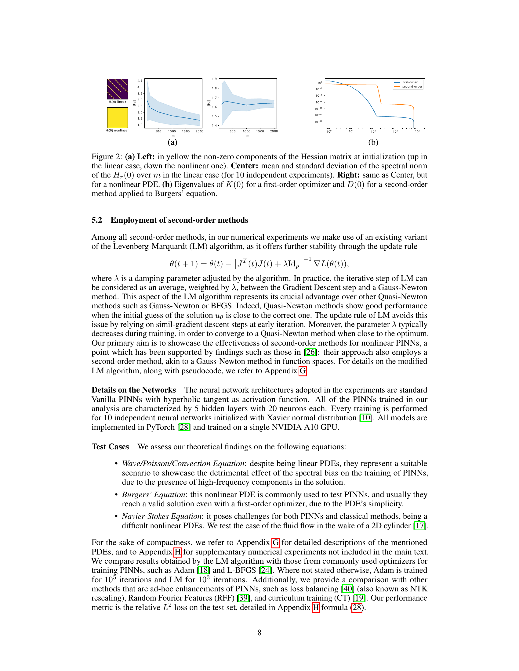
🔼 Figure 3 shows the results of applying different optimizers (Adam, LM, LBFGS) to solve the Poisson and Convection equations. Part (a) compares the median and standard deviation of the relative L2 loss over training iterations for the Poisson equation. Part (b) presents a comparison for the Convection equation, showing the median and standard deviation of the L2 loss after 1000 iterations with and without curriculum training (CT), for various convection coefficients (β). A sample solution obtained using the Levenberg-Marquardt (LM) optimizer after 5000 iterations with β=100 is also displayed.
read the caption
Figure 3: (a) Poisson equation: median and standard deviation of the relative L2 loss for different optimizers over training iterations (repetitions over 10 independent runs). (b) Convection equation: median and standard deviation of the L2 loss after 1000 iterations achieved over 5 independent runs with and without CT for different values of the convection coefficient β (left) and solution obtained with LM (and no other enhancement) after 5000 iterations with β = 100 (right).

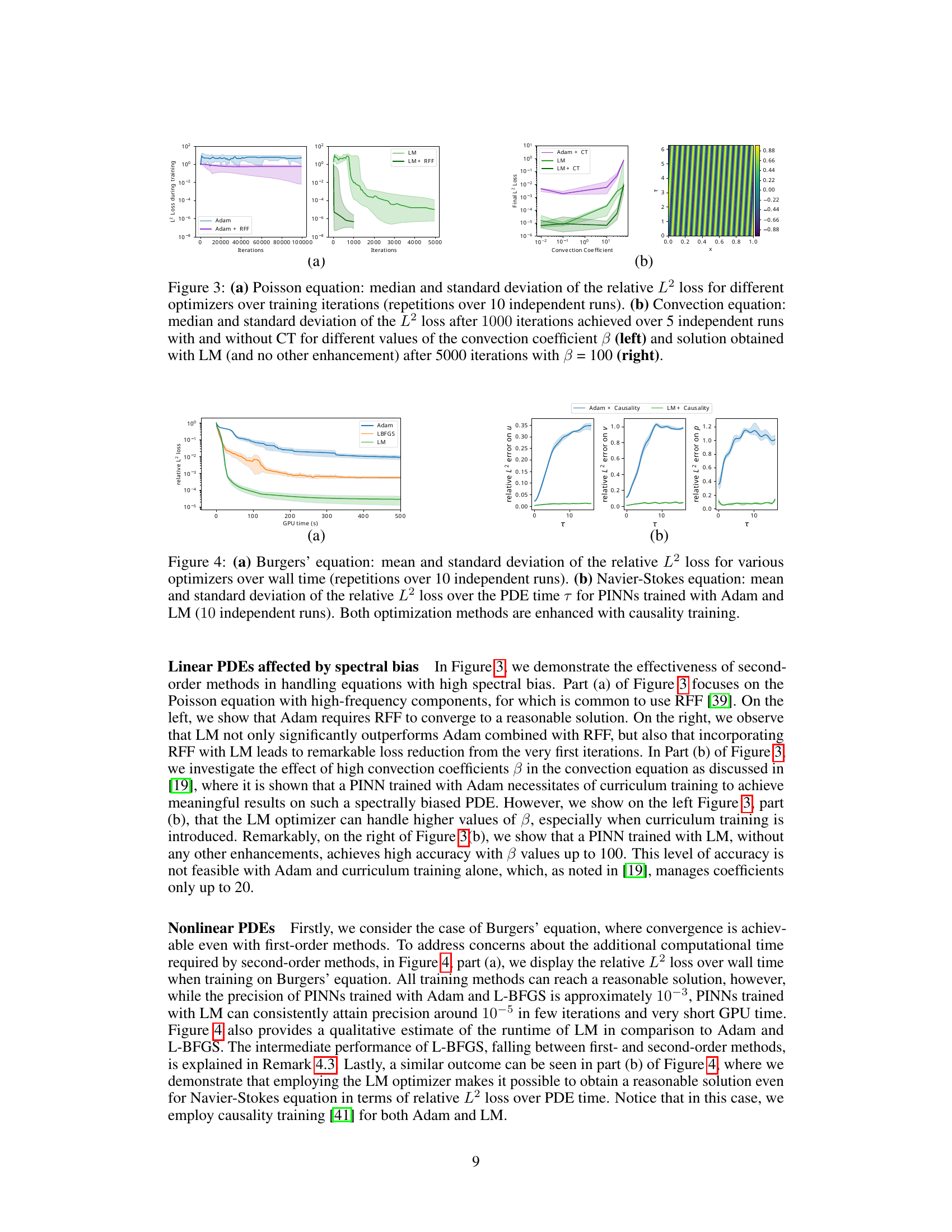
🔼 This figure compares the performance of Adam and LM optimizers on Burgers’ and Navier-Stokes equations. Part (a) shows the relative L2 loss against wall time (computational time) for both optimizers on the Burgers’ equation, highlighting LM’s faster convergence. Part (b) illustrates the relative L2 error over time (τ) for both optimizers on the Navier-Stokes equation, showcasing the superior accuracy of LM, particularly in approximating velocity and pressure. Both optimizers incorporated causality training in this experiment.
read the caption
Figure 4: (a) Burgers' equation: mean and standard deviation of the relative L2 loss for various optimizers over wall time (repetitions over 10 independent runs). (b) Navier-Stokes equation: mean and standard deviation of the relative L2 loss over the PDE time τ for PINNs trained with Adam and LM (10 independent runs). Both optimization methods are enhanced with causality training.

🔼 This figure displays the performance of three different optimization algorithms (Adam, L-BFGS, and LM) on a wave equation. The y-axis shows the relative L2 loss on a test set, and the x-axis represents the number of iterations during training. The plot shows the mean relative L2 loss for each algorithm across 10 independent runs, along with error bars representing the standard deviation. The results demonstrate the comparative performance of these optimizers in minimizing the loss function for the wave equation.
read the caption
Figure 5: Mean and standard deviation of the relative L2 loss on the test set on the Wave equation for Adam, L-BFGS and LM optimizer over iterations (repetition over 10 independent runs).

🔼 This figure shows the results of experiments on the Wave equation. Three contour plots are displayed, each representing the predicted solution of a Physics-Informed Neural Network (PINN) trained using different optimization methods. The left plot shows the result obtained using the Adam optimizer, while the center plot shows the result obtained using the Levenberg-Marquardt (LM) optimizer. The right plot displays the true solution. The plots are presented to visually compare the accuracy of PINNs trained with different optimizers in solving the Wave equation.
read the caption
Figure 6: Experiments on the Wave equation. Left: Prediction of the parametrized solution of a PINN trained with Adam (Left) and LM (Center) alongside with the true solution (Right).
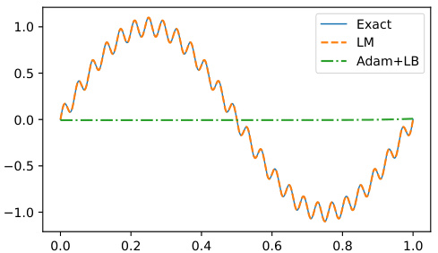
🔼 This figure compares the prediction of the solution of the Poisson equation using three different methods: Levenberg-Marquardt (LM), Adam with loss balancing (Adam+LB), and the exact solution. It visually demonstrates the performance differences between LM and Adam+LB, showing that LM achieves greater accuracy in approximating the true solution.
read the caption
Figure 7: Experiments on the prediction of the solution of Poisson equation with LM and Adam (with loss balancing), both compared with the exact solution.
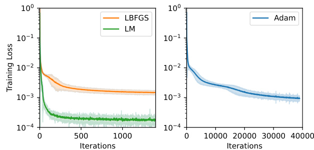
🔼 This figure compares the training loss curves for three different optimization algorithms (Adam, LBFGS, and LM) when applied to the Navier-Stokes equation. The plot shows that LM consistently achieves a lower training loss compared to the other two methods. Error bars representing standard deviation across 10 independent runs are included for each method, demonstrating the variability in performance across different random initializations. The y-axis is logarithmic scale for training loss, showing the range of loss values across multiple runs.
read the caption
Figure 8: Mean and standard deviation of the training loss over the iterations for Adam, LBFGS and LM on Navier-Stokes equation (for 10 independent runs).
Full paper#

