TL;DR#
Estimating optical flow, crucial for understanding motion in videos, is computationally expensive, particularly with multi-frame methods that repeatedly estimate flow between pairs of frames. This leads to redundancy and slow processing. Existing multi-frame methods also struggle to effectively model the complex interactions between spatial and temporal information in videos, hindering accuracy.
StreamFlow tackles this by introducing a streamlined in-batch multi-frame pipeline that simultaneously predicts flows for multiple frames within a single pass, significantly reducing redundancy and speeding up processing. It also introduces novel spatiotemporal modeling techniques, ISC and GTR, that efficiently capture both spatial and temporal information, leading to significant improvements in accuracy, especially in difficult areas such as occluded regions. Experimental results demonstrate that StreamFlow achieves substantial improvements in both speed and accuracy compared to existing methods on several benchmark datasets. The method shows strong cross-dataset generalization abilities, further demonstrating its robustness and wider applicability.
Key Takeaways#
Why does it matter?#
This paper is important because it presents StreamFlow, a novel approach to optical flow estimation that significantly improves speed and accuracy. Its streamlined multi-frame pipeline and innovative spatiotemporal modeling techniques offer substantial advancements over existing methods. This opens new avenues for research in video processing and related computer vision tasks, particularly those requiring real-time performance or dealing with high-resolution videos.
Visual Insights#

🔼 This figure compares the traditional pairwise multi-frame optical flow estimation pipeline with the proposed streamlined in-batch multi-frame (SIM) pipeline. The pairwise approach estimates flow repeatedly for each pair of consecutive frames, leading to redundant calculations. In contrast, the SIM pipeline predicts all successive unidirectional flows in a single forward pass, thereby minimizing redundant computations and improving efficiency. The dashed lines highlight the additional computations required by the pairwise method.
read the caption
Figure 1: Comparison between the pairwise and the proposed Streamlined In-batch Multi-frame (SIM) pipeline. Short dashed lines represent additional computations.

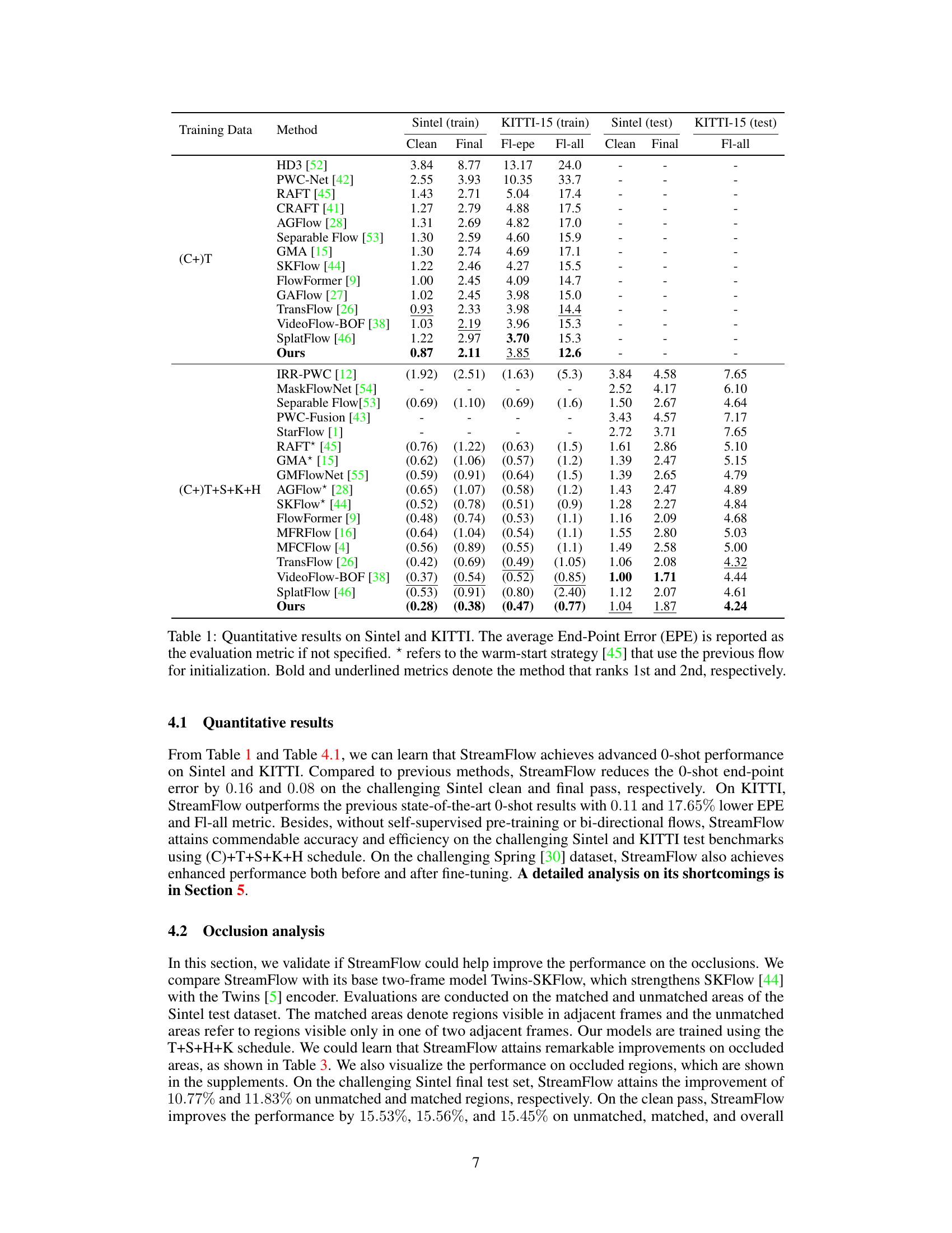
🔼 This table presents a quantitative comparison of StreamFlow against various state-of-the-art optical flow estimation methods on the Sintel and KITTI datasets. It shows the end-point error (EPE) for both clean and final passes of the Sintel dataset, along with the all, clean and final evaluations for KITTI. The table also highlights the performance of methods using a warm-start strategy, indicating the use of prior flow information.
read the caption
Table 1: Quantitative results on Sintel and KITTI. The average End-Point Error (EPE) is reported as the evaluation metric if not specified. * refers to the warm-start strategy [45] that use the previous flow for initialization. Bold and underlined metrics denote the method that ranks 1st and 2nd, respectively.
In-depth insights#
SIM Pipeline Speedup#
The Streamlined In-batch Multi-frame (SIM) pipeline significantly accelerates multi-frame optical flow estimation by minimizing redundant computations. Instead of processing frames pairwise, which necessitates repeated flow calculations for consecutive frames, the SIM pipeline processes multiple frames simultaneously in a single forward pass, resulting in a substantial speedup. This is achieved by intelligently structuring the input such that each batch yields a sequence of unidirectional flows. While the theoretical speedup is proportional to the number of frames, practical improvements frequently exceed this due to the reduced memory access and data transfer overhead. The efficiency gains from SIM are further enhanced by the algorithm’s design, which minimizes pairwise spatiotemporal modeling and leverages efficient spatiotemporal coherence modeling techniques. This combination of structural optimization and efficient modeling makes SIM a key element in StreamFlow’s superior speed and accuracy compared to traditional multi-frame methods.
ISC/GTR Enhancements#
The paper introduces two novel modules, ISC (Integrative Spatiotemporal Coherence) and GTR (Global Temporal Regressor), to significantly enhance the accuracy and efficiency of optical flow estimation. ISC, embedded in the encoder, leverages spatiotemporal relationships effectively without adding extra parameters, improving performance, particularly in challenging areas such as occlusions. GTR, part of the decoder, refines optical flow predictions through lightweight temporal modeling, further boosting accuracy. The combination of ISC and GTR within the streamlined SIM pipeline leads to considerable improvements over baseline methods, showcasing the modules’ effectiveness in capturing rich spatiotemporal context and minimizing computational redundancies. The parameter efficiency of ISC is especially noteworthy, offering a significant advantage in terms of computational resource utilization. The results demonstrate that these integrated modules contribute substantially to the overall accuracy gains observed in the experiments.
Cross-Dataset Robustness#
Cross-dataset robustness is a critical aspect of evaluating the generalizability of a model. A model demonstrating strong cross-dataset robustness performs well on datasets beyond those used for training, indicating its ability to handle variations in data distribution, image quality, and annotation styles. This robustness is crucial for real-world deployment, as models are unlikely to encounter data that perfectly matches the training distribution. Analyzing cross-dataset performance requires careful consideration of various factors, including the choice of target datasets which must exhibit sufficient differences to reveal limitations, appropriate evaluation metrics, and a clear understanding of the model’s strengths and weaknesses. A high degree of cross-dataset robustness suggests that the underlying learned representations are not overly specialized to the training data, implying a more fundamental understanding of the problem. However, low performance on unseen datasets should not immediately signal failure, as the model may just lack the specific features or data characteristics needed for optimal results within the new dataset, requiring further investigation or modifications. Ultimately, comprehensive cross-dataset evaluations are essential to ascertain a model’s true capacity and reliability.
Occlusion Handling#
Effective occlusion handling is crucial for robust optical flow estimation, as occlusions disrupt the apparent motion of objects. Many methods address this by incorporating temporal context, leveraging information from multiple frames to infer motion behind occluded regions. Spatiotemporal modeling is often employed, integrating spatial and temporal features to better predict flow in areas where direct correspondence is missing. Techniques like motion feature compensation or the use of occlusion maps help to identify and mitigate the impact of occlusions. Advanced approaches may integrate bidirectional flow estimation, utilizing both forward and backward flow predictions to improve accuracy in challenging scenarios. Some methods directly model the uncertainty introduced by occlusions, using probabilistic or variational methods to represent the ambiguity inherent in these areas. Parameter efficiency is a significant consideration, as complex models can slow down inference. Therefore, lightweight and computationally efficient methods for occlusion handling are often preferred for real-time or resource-constrained applications. The success of any occlusion handling technique heavily depends on the characteristics of the input video and the tradeoff between accuracy and computational cost.
Future Work: Memory#
Future work in memory optimization for optical flow estimation could explore several promising avenues. Reducing memory footprint is crucial, especially for handling high-resolution videos and long sequences. Techniques like efficient data structures, compression algorithms, and memory-aware training strategies (e.g., gradient checkpointing) should be investigated. Improving memory access efficiency is vital, as memory bandwidth often becomes a bottleneck. Optimizations in data layout, prefetching schemes, and hardware-accelerated memory management could significantly enhance performance. Furthermore, research into novel memory architectures tailored to the specific needs of optical flow estimation, such as specialized hardware accelerators or hierarchical memory systems, warrants attention. Exploring alternative memory models that move beyond traditional RAM and leverage persistent memory or other non-volatile memory technologies could enable processing of massive datasets without significant performance degradation. Finally, developing sophisticated algorithms that can effectively manage memory usage dynamically, adapting to the characteristics of each video sequence, would be a major advancement.
More visual insights#
More on figures
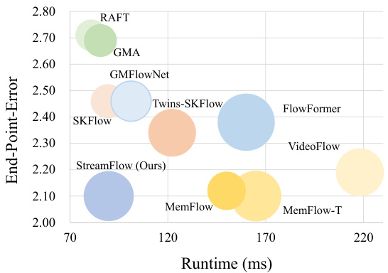
🔼 This figure compares the performance (end-point error) and efficiency (runtime in milliseconds) of different optical flow estimation methods. The size of each bubble represents the number of parameters in the model. All models were trained using the (C+)T schedule and evaluated on the Sintel final pass dataset. The figure highlights the trade-off between accuracy and speed, showing that StreamFlow achieves state-of-the-art performance with comparable efficiency to simpler two-frame methods.
read the caption
Figure 2: Comparison between performance and efficiency. A larger bubble denotes more parameters. Models are trained via the (C+)T schedule and tested on the Sintel final pass.

🔼 This figure provides a detailed overview of the StreamFlow architecture. Panel (a) shows the overall framework, highlighting the Twins transformer encoder, the cost volume calculation (limited to adjacent frames for efficiency), and the iterative GTR decoder. The dot product operation is also indicated. Panel (b) zooms in on the iterative GTR decoder, illustrating the motion encoder, temporal and spatial feature integration, the motion updater, and how flows are refined iteratively. The key point is the streamlined multi-frame processing, avoiding redundant computation.
read the caption
Figure 3: Overview of StreamFlow. (a) illustrates the overall framework and <,> denotes the dot-product operation. The computation of cost volume is limited to adjacent frames and is performed once in one forward pass. Flows are initialized to zeros. (b) depicts the details of the GTR decoder.

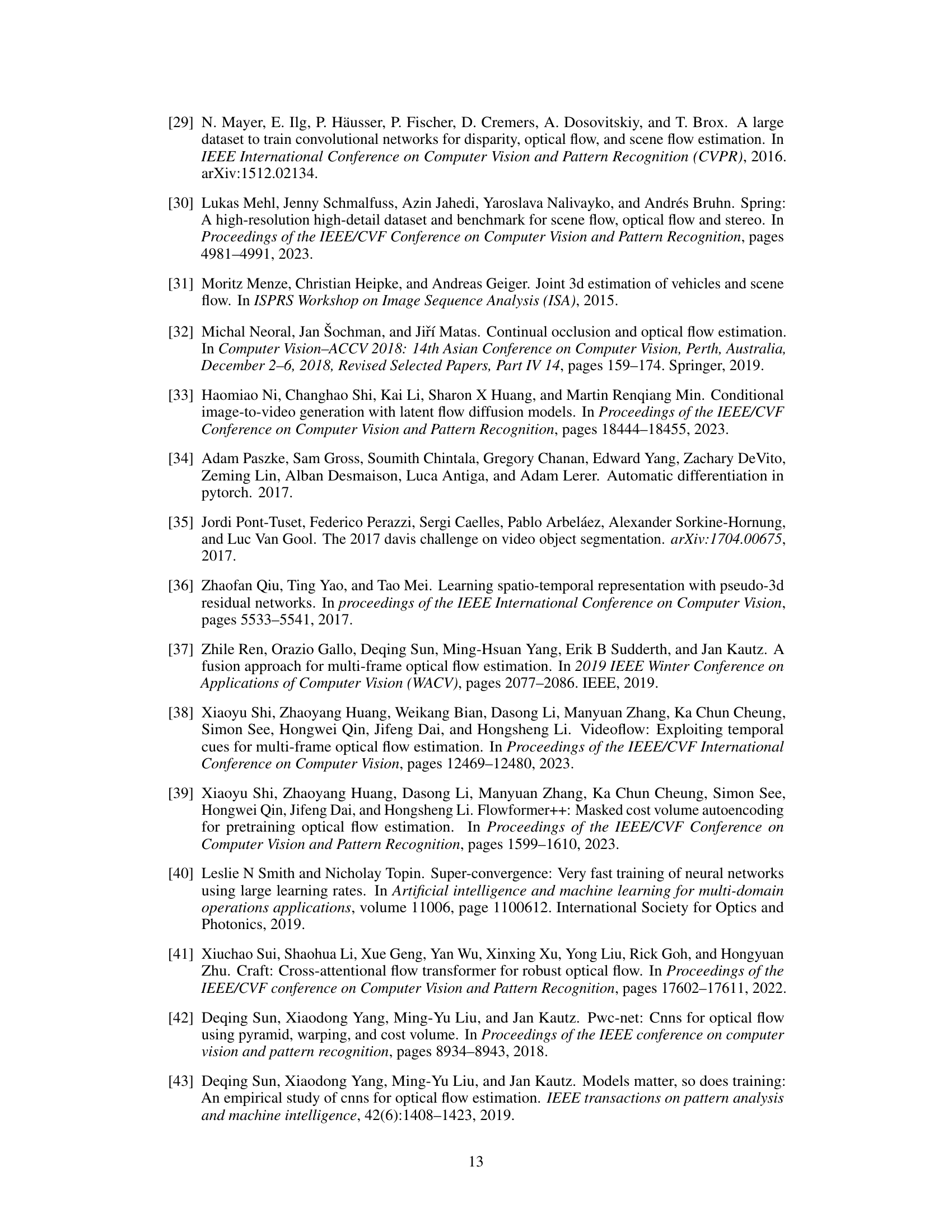
🔼 This figure shows a comparison of optical flow estimation results between the baseline method (Twins-SKFlow) and the proposed StreamFlow method on both synthetic (Sintel) and real-world (KITTI) datasets. The red boxes highlight areas where StreamFlow shows improved performance, indicating fewer artifacts and more accurate flow predictions, especially in challenging areas like occluded regions. The figure demonstrates StreamFlow’s ability to generalize well to different types of video data.
read the caption
Figure 4: Visualizations of results on Sintel and KITTI test sets. Differences are highlighted with red bounding boxes. StreamFlow achieves fewer artifacts on both synthetic and real-world scenes. More visualization results on DAVIS [35] and occluded regions are in the supplements.

🔼 This figure shows visual comparisons of optical flow estimation results between StreamFlow and a baseline method on the Sintel and KITTI datasets. The top row shows input image pairs, and the bottom row shows the corresponding optical flow estimations. Red boxes highlight areas where StreamFlow shows improved performance, namely fewer artifacts, suggesting better accuracy in capturing fine details and movement, especially in real-world scenes. Supplementary material includes more visualizations, including results on the DAVIS dataset and in occluded regions.
read the caption
Figure 4: Visualizations of results on Sintel and KITTI test sets. Differences are highlighted with red bounding boxes. StreamFlow achieves fewer artifacts on both synthetic and real-world scenes. More visualization results on DAVIS [35] and occluded regions are in the supplements.

🔼 This figure visualizes the performance of StreamFlow and VideoFlow on occluded regions of the Sintel dataset. Occlusion maps highlight the occluded areas. The flow error maps show the error between the estimated flow and the ground truth flow. The results demonstrate that StreamFlow achieves significantly lower errors in occluded regions than VideoFlow, indicating its improved performance in handling occlusions.
read the caption
Figure 6: Visualizations of the performance on the occluded regions. StreamFlow achieves comparable performance even with advanced methods. All models are trained on the FlyingThings dataset. A darker color in the flow error map denotes a higher estimation error compared with ground truth.
More on tables
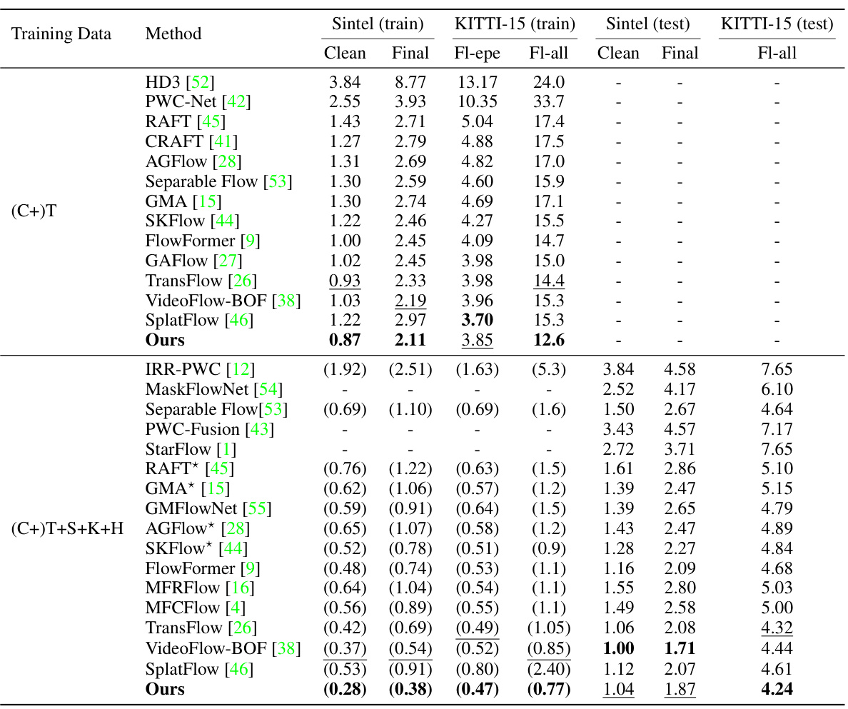
🔼 This table presents a quantitative comparison of StreamFlow against other state-of-the-art methods on the Sintel and KITTI datasets. The results are broken down by dataset (Sintel and KITTI), and further by test set (Clean and Final for Sintel). The main metric used is End-Point Error (EPE), representing the average error in predicted optical flow. The table also indicates whether a warm-start strategy was used (using the previous flow for initialization). The best and second-best performing methods in each category are highlighted.
read the caption
Table 1: Quantitative results on Sintel and KITTI. The average End-Point Error (EPE) is reported as the evaluation metric if not specified. * refers to the warm-start strategy [45] that use the previous flow for initialization. Bold and underlined metrics denote the method that ranks 1st and 2nd, respectively.

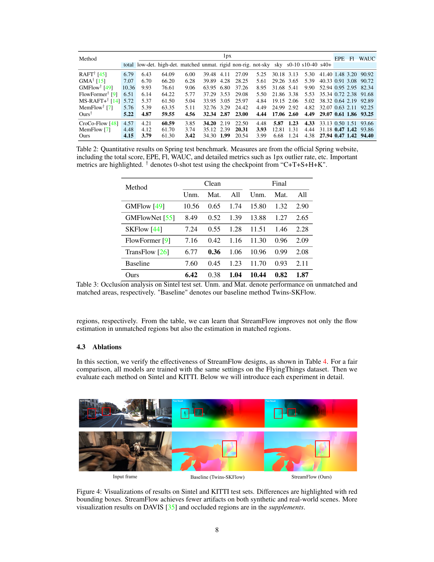
🔼 This table presents a quantitative comparison of various optical flow methods on the Spring benchmark dataset. It includes the total score (a summary metric), EPE (End-Point Error), FI (F-measure), and WAUC (weighted area under the curve). Detailed metrics are also provided, such as the percentage of outliers with 1-pixel error, along with breakdowns for low- and high-detection difficulty, matched and unmatched regions, rigid and non-rigid motions, and sky and non-sky regions. The results are shown for different thresholds for flow errors. Note that the results marked with † are obtained by performing a 0-shot test (evaluating the model without fine-tuning on the Spring dataset itself).
read the caption
Table 2: Quantitative results on Spring test benchmark. Measures are from the official Spring website, including the total score, EPE, FI, WAUC, and detailed metrics such as 1px outlier rate, etc. Important metrics are highlighted. † denotes 0-shot test using the checkpoint from “C+T+S+H+K”.
🔼 This table presents a comparison of the StreamFlow model’s performance against other state-of-the-art optical flow estimation methods on the Sintel and KITTI datasets. The performance is measured using the average End-Point Error (EPE), a common metric for optical flow accuracy. The table also shows results for different test sets (clean and final) within each dataset and highlights the top two performing methods for each metric.
read the caption
Table 1: Quantitative results on Sintel and KITTI. The average End-Point Error (EPE) is reported as the evaluation metric if not specified. * refers to the warm-start strategy [45] that use the previous flow for initialization. Bold and underlined metrics denote the method that ranks 1st and 2nd, respectively.
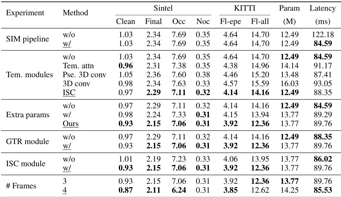
🔼 This table presents the ablation study of the proposed StreamFlow model. It systematically evaluates the impact of different components of the model, namely, the SIM pipeline, temporal modules, extra parameters, GTR module, and ISC module, on the model’s performance. The results are presented in terms of End-Point Error (EPE) metrics on both Sintel and KITTI datasets, along with the number of parameters (M) and latency (ms). The underlined results indicate the final model configuration.
read the caption
Table 4: Ablations on our proposed design. All models are trained using the 'C+T' schedule. The number of refinements is 12 for all methods. The settings used in our final model are underlined.

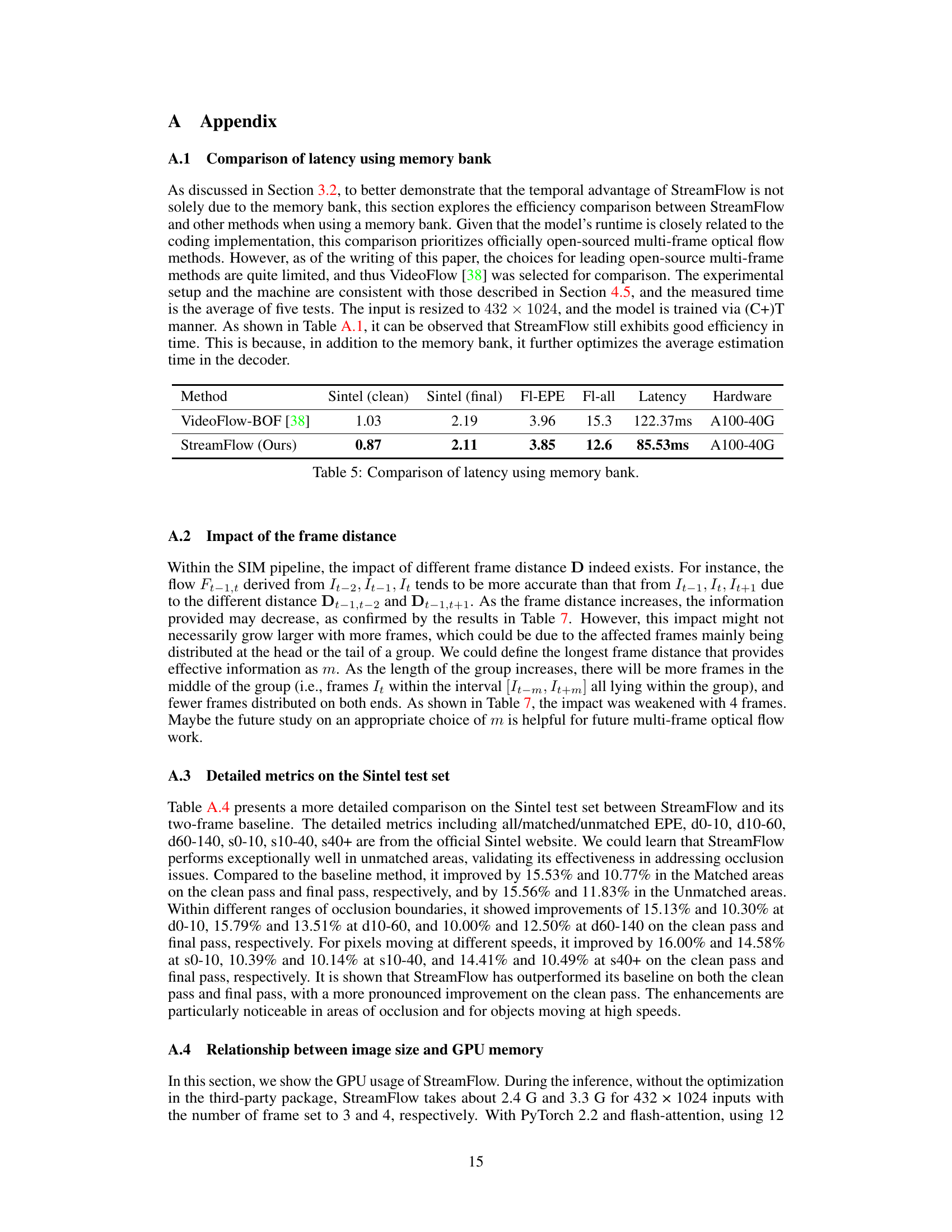
🔼 This table compares the latency of VideoFlow-BOF and StreamFlow when using a memory bank. The comparison highlights the efficiency gains achieved by StreamFlow, showing a significant reduction in latency despite using a memory bank. It emphasizes the efficiency improvements of StreamFlow are not solely attributed to memory bank usage but also to optimizations in the decoder.
read the caption
Table 5: Comparison of latency using memory bank.

🔼 This table presents a comparison of the proposed StreamFlow model against other state-of-the-art methods for optical flow estimation on the Sintel and KITTI datasets. It shows the performance (End-Point Error or EPE) of various methods under different training data conditions. The results are broken down by dataset (Sintel clean, Sintel final, KITTI15), and further separated into overall performance, and performance on occluded regions. The table highlights the top-performing methods.
read the caption
Table 1: Quantitative results on Sintel and KITTI. The average End-Point Error (EPE) is reported as the evaluation metric if not specified. * refers to the warm-start strategy [45] that use the previous flow for initialization. Bold and underlined metrics denote the method that ranks 1st and 2nd, respectively.
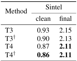
🔼 This table shows the impact of using different numbers of frames (3 and 4) and different frame distances on the performance of the StreamFlow model. The results are evaluated on the Sintel dataset using two metrics: clean and final. The ‘+’ symbol indicates the use of nearer frames, suggesting that using frames closer together might improve accuracy in some cases.
read the caption
Table 7: Impact of frame distance. † denotes using nearer frames.

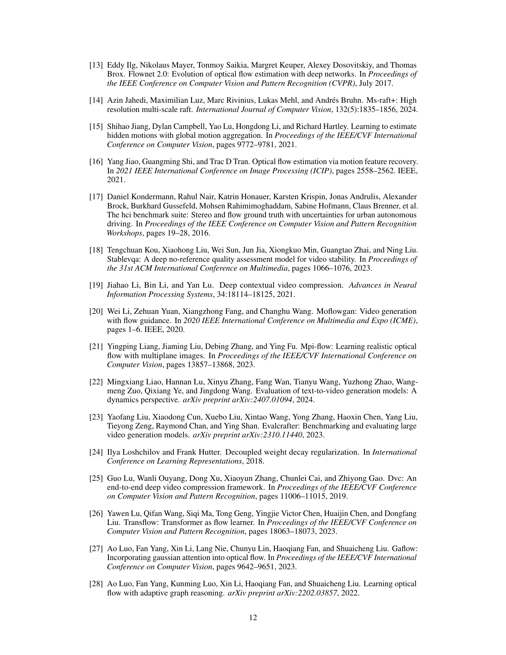
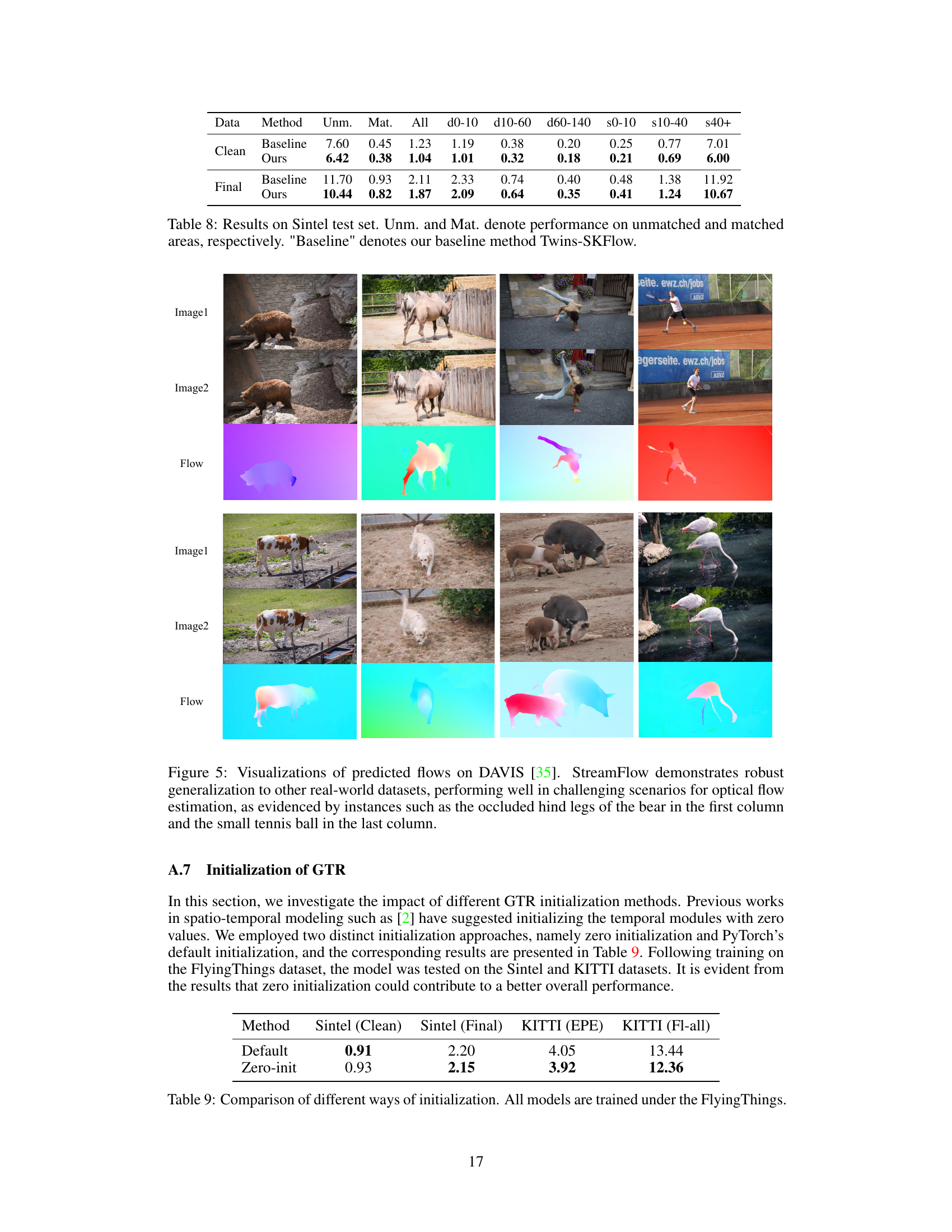
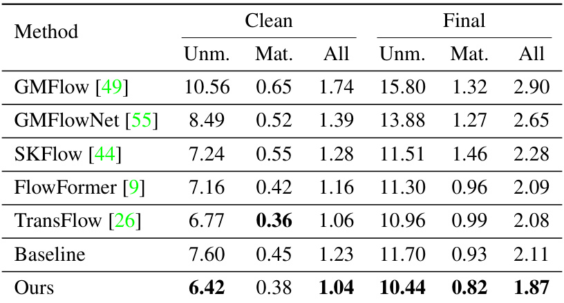
🔼 This table presents a detailed comparison of the performance of the proposed StreamFlow model and its baseline (Twins-SKFlow) on the Sintel test dataset. It breaks down the results (End-Point Error or EPE) for various motion characteristics: unmatched areas (regions where motion is only visible in one of two frames), matched areas (motion visible in both frames), and across different ranges of motion speed. The results highlight StreamFlow’s improved accuracy, particularly in challenging unmatched areas.
read the caption
Table 8: Results on Sintel test set. Unm. and Mat. denote performance on unmatched and matched areas, respectively. 'Baseline' denotes our baseline method Twins-SKFlow.

🔼 This table compares the performance of different initialization methods for the GTR (Global Temporal Regressor) module in the StreamFlow model. The models were trained using the FlyingThings dataset, and the results are evaluated on the Sintel and KITTI datasets using End-Point Error (EPE) and the overall flow error metric (Fl-all). The comparison highlights the impact of different initialization strategies on model performance.
read the caption
Table 9: Comparison of different ways of initialization. All models are trained under the FlyingThings.
Full paper#


