TL;DR#
Training neural networks efficiently and effectively is a major challenge. A key hyperparameter is the learning rate (LR), which controls the size of the steps taken during optimization. While using large LRs initially is common practice to avoid poor local minima and improve generalization, there’s limited understanding on exactly how large is optimal and what the differences in the resulting models are. This paper aims to address this gap.
The researchers conducted a controlled experiment by fixing the initial LR and exploring its effect on model performance. They found that only a narrow range of initial LRs, just above the convergence threshold, consistently led to the best results after fine-tuning or weight averaging. Models trained with these optimal LRs exhibited high-quality minima, and only focused on relevant features in the dataset. Using either too small or too large initial LRs yielded suboptimal results. These findings provide valuable insights into the dynamics of neural network training, particularly in choosing the right initial learning rates, and offer practical guidance for researchers.
Key Takeaways#
Why does it matter?#
This paper is crucial because it offers practical guidance on using large learning rates, a common practice in deep learning that often lacks precise benchmarks. It bridges the gap between theory and practice by providing insights into optimal learning rate ranges, the geometry of solutions, and feature learning. This is highly relevant to improving training efficiency and generalization, impacting a broad range of deep learning applications. Researchers can directly apply the findings to enhance their models’ performance and explore new avenues in optimization and feature selection.
Visual Insights#

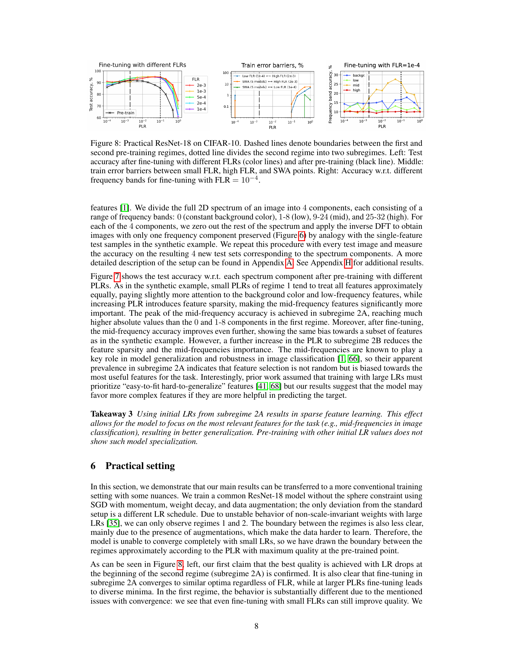
🔼 This figure shows the test accuracy of a scale-invariant ResNet-18 model trained on CIFAR-10 with different fixed learning rates (LRs). It illustrates three distinct training regimes identified by the authors: 1) convergence (low LRs where the model monotonically converges to a minimum), 2) chaotic equilibrium (medium LRs where the loss noisily stabilizes), and 3) divergence (high LRs leading to random-guess accuracy). The dashed lines separate these regimes, and the plot displays the mean test accuracy and standard deviation over the last 20 of 200 training epochs. This is a key figure in establishing the three training regimes which are central to the paper’s experimental methodology.
read the caption
Figure 1: Three regimes of training with a fixed LR. Mean test accuracy + standard deviation on the last 20 out of 200 epochs are shown. Dashed lines denote boundaries between the training regimes. SI ResNet-18 on CIFAR-10.
In-depth insights#
Optimal LR Range#
The concept of an optimal learning rate (LR) range is crucial for effective neural network training. The paper investigates the impact of different initial LRs on model generalization and feature learning. It identifies a narrow range of initial LRs, slightly exceeding the convergence threshold, that consistently yields superior results after fine-tuning or weight averaging. This optimal range allows the optimization process to locate a basin containing only high-quality minima, as opposed to unstable minima found with smaller LRs or basins lacking good solutions found with larger LRs. Furthermore, initial LRs within the optimal range promote a sparse set of learned features, focusing on those most relevant for the task, unlike the less selective feature learning observed with both suboptimal LR choices. The study underscores that simply using a large LR is insufficient; rather, a precise and well-defined range, carefully chosen based on the specifics of the network and task, is key to achieving optimal performance. The existence of this optimal range highlights the complex interplay between LR, optimization dynamics, and generalization. Further research should focus on generalizing the findings beyond specific network architectures and datasets and on establishing more robust methods for identifying the optimal LR range.
Loss Landscape Geom#
Analyzing the loss landscape geometry offers crucial insights into the optimization process of neural networks. The ‘Loss Landscape Geom’ section would ideally explore the characteristics of the minima reached after training with varying learning rates. This involves investigating the curvature and connectivity of these minima, determining whether they form clusters or basins, and analyzing the relationships between the geometry and the generalization ability of the resulting models. A key aspect would be to compare the geometry of minima obtained with large learning rates versus those achieved with small learning rates, revealing differences that might explain the observed superior generalization of models trained with large initial rates. Furthermore, the analysis could delve into the relationship between local and global minima, assessing if large rates facilitate escaping poor local minima and reaching regions of better solutions. Finally, this section could include visualizations of the loss landscape, showcasing the pathways taken during training and providing quantitative measures of curvature and connectivity to support the presented findings. Such a comprehensive analysis would offer deeper understanding of why large learning rates are beneficial.
Feature Sparsity#
The concept of feature sparsity, explored in the context of neural network training with varying learning rates, reveals crucial insights into model behavior and generalization. Higher initial learning rates, within an optimal range, promote the learning of a sparse subset of features, focusing on those most relevant to the task. This sparsity isn’t merely a byproduct; it’s linked to the location of high-quality minima in the loss landscape. Conversely, training with excessively small or large initial learning rates leads to dense feature learning, unstable minima, and poor generalization. The optimal learning rate range seems to strike a balance, avoiding both the underfitting of overly simplistic models (small LRs) and the overfitting resulting from learning too many potentially irrelevant features (large LRs). Feature sparsity appears essential for achieving both good generalization and locating these beneficial minima. The observed feature sparsity suggests that the model is more specialized and efficient in its representation of data, which is a key factor in its improved ability to generalize.
Practical Setting#
The heading ‘Practical Setting’ in a research paper usually signifies a shift from controlled experiments to real-world application. It suggests the authors are testing their findings in a less-controlled environment, evaluating the robustness and generalizability of their approach. This section would likely demonstrate the method’s performance on standard datasets or in a setting more closely resembling actual usage scenarios. Key aspects within this section would include comparing results obtained in the practical setting with those from the controlled experiments. Any discrepancies could provide valuable insights into the limits of the method’s applicability. Additionally, a comparison would highlight aspects like the impact of noisy data, data heterogeneity, and the presence of confounding factors, as these are absent or minimized in controlled settings. The success of the method in the practical setting is a crucial test of its broader utility and value. It confirms the method’s ability to provide comparable or improved results even under less ideal circumstances, demonstrating its true potential for practical use. Finally, it could discuss challenges encountered during implementation and potential modifications or adaptations made to suit the practical setting. This section is crucial for assessing the practical relevance and impact of the research findings.
Future Research#
The paper’s ‘Future Research’ section could fruitfully explore several avenues. A deeper theoretical understanding of the observed empirical phenomena is crucial. Why does a specific range of learning rates consistently yield superior results? Is there a fundamental mathematical relationship between the loss landscape’s geometry and the resulting feature sparsity? Further investigation into the role of model architecture is warranted. Do these findings generalize across various network depths, widths, and activation functions? A more thorough examination of practical LR scheduling strategies is needed to bridge the gap between controlled experiments and real-world training protocols. The interaction between LR, normalization techniques, and other hyperparameters requires further study. Finally, expanding the scope of applications beyond image classification to other domains like natural language processing and time series analysis will validate the robustness and generality of the key findings.
More visual insights#
More on figures

🔼 This figure shows the test accuracy results for fine-tuned and SWA models on the CIFAR-10 dataset using a scale-invariant ResNet-18. The left panel displays the results from fine-tuning with different fine-tuning learning rates (FLRs), while the right panel shows the results obtained through SWA with varying numbers of models. The black line in both panels represents the test accuracy achieved after pre-training with different pre-training learning rates (PLRs). The dashed vertical lines separate the three training regimes identified in the paper (convergence, chaotic equilibrium, and divergence), and the dotted line further subdivides the second regime (chaotic equilibrium) into two sub-regimes (2A and 2B). The figure demonstrates how the choice of initial LR impacts the final model performance after fine-tuning or SWA.
read the caption
Figure 2: Test accuracy of the fine-tuned (left) and SWA (right) solutions for SI ResNet-18 on CIFAR-10. Test accuracy after pre-training is depicted with the black line. Dashed lines denote boundaries between the pre-training regimes, dotted line divides the second regime into two subregimes.

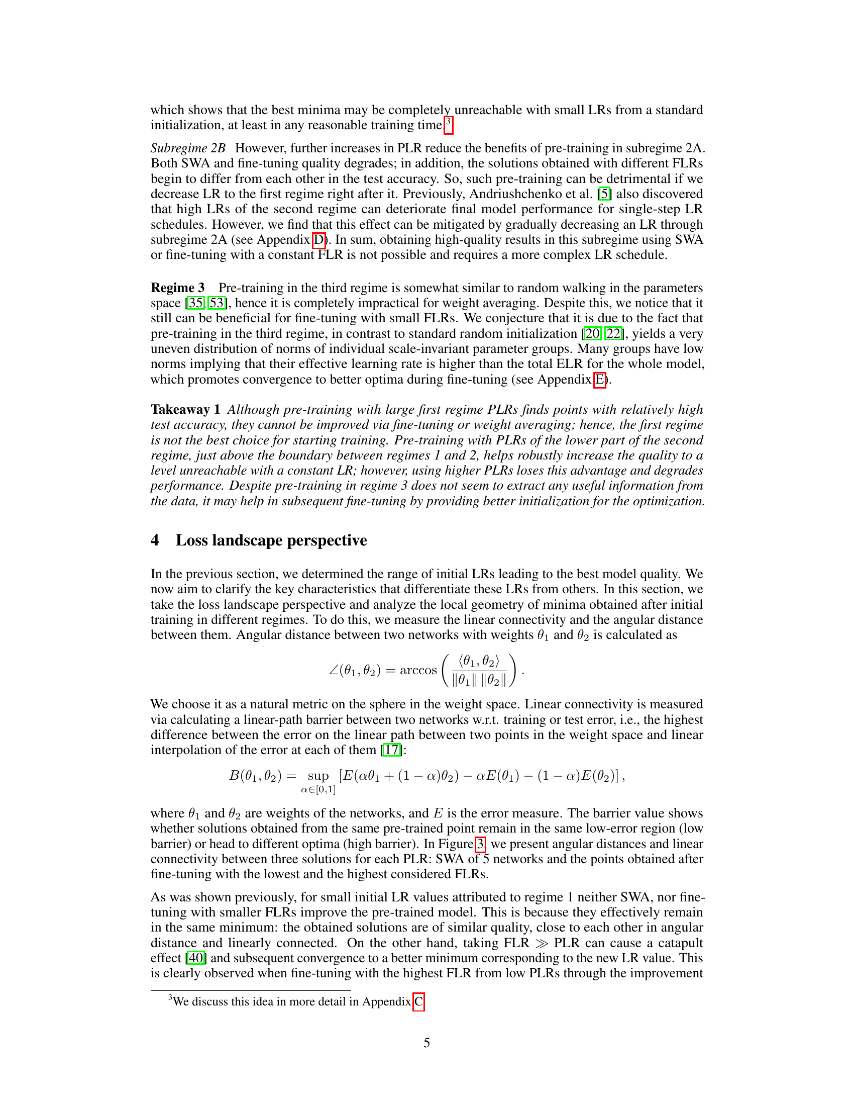
🔼 This figure visualizes the relationship between different solutions obtained after pre-training with various learning rates (PLRs) and subsequent fine-tuning with either small or large fine-tuning learning rates (FLRs) or by using Stochastic Weight Averaging (SWA). It displays three plots: angular distance, train error barriers, and test error barriers. The plots show the angular distance (a measure of the difference in model weights) and the linear error barrier (a measure of the connectivity of low-error solutions) between the smallest FLR, the largest FLR, and the SWA method for each PLR. This helps to understand the landscape of the loss function around minima reached by different training regimes.
read the caption
Figure 3: Geometry between the points fine-tuned with the smallest and the largest FLRs and SWA. SI ResNet-18 on CIFAR-10.

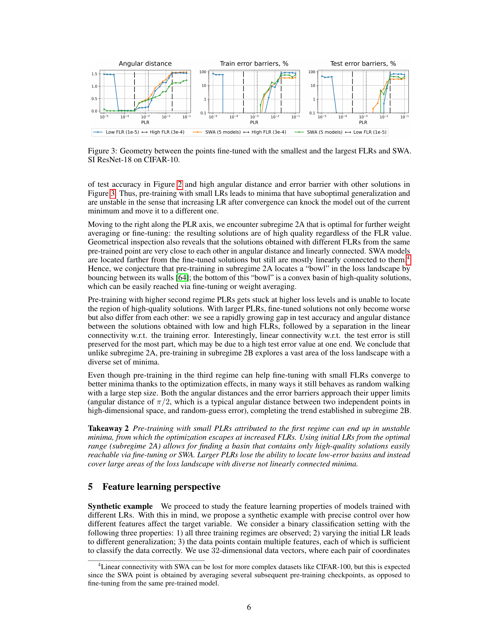
🔼 This figure shows a single 2D ’tick’ feature used in the synthetic example. The x and y axes represent the two dimensions of the feature. The dots represent data points, colored red for class 0 and blue for class 1. The data points are scattered in a pattern designed such that each coordinate of the feature is sufficient to perform binary classification. This pattern allows the researchers to study how the model learns features in different training regimes.
read the caption
Figure 4: A single 2D 'tick' feature used in the synthetic example.
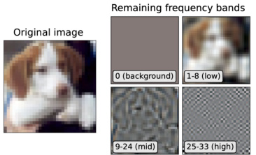
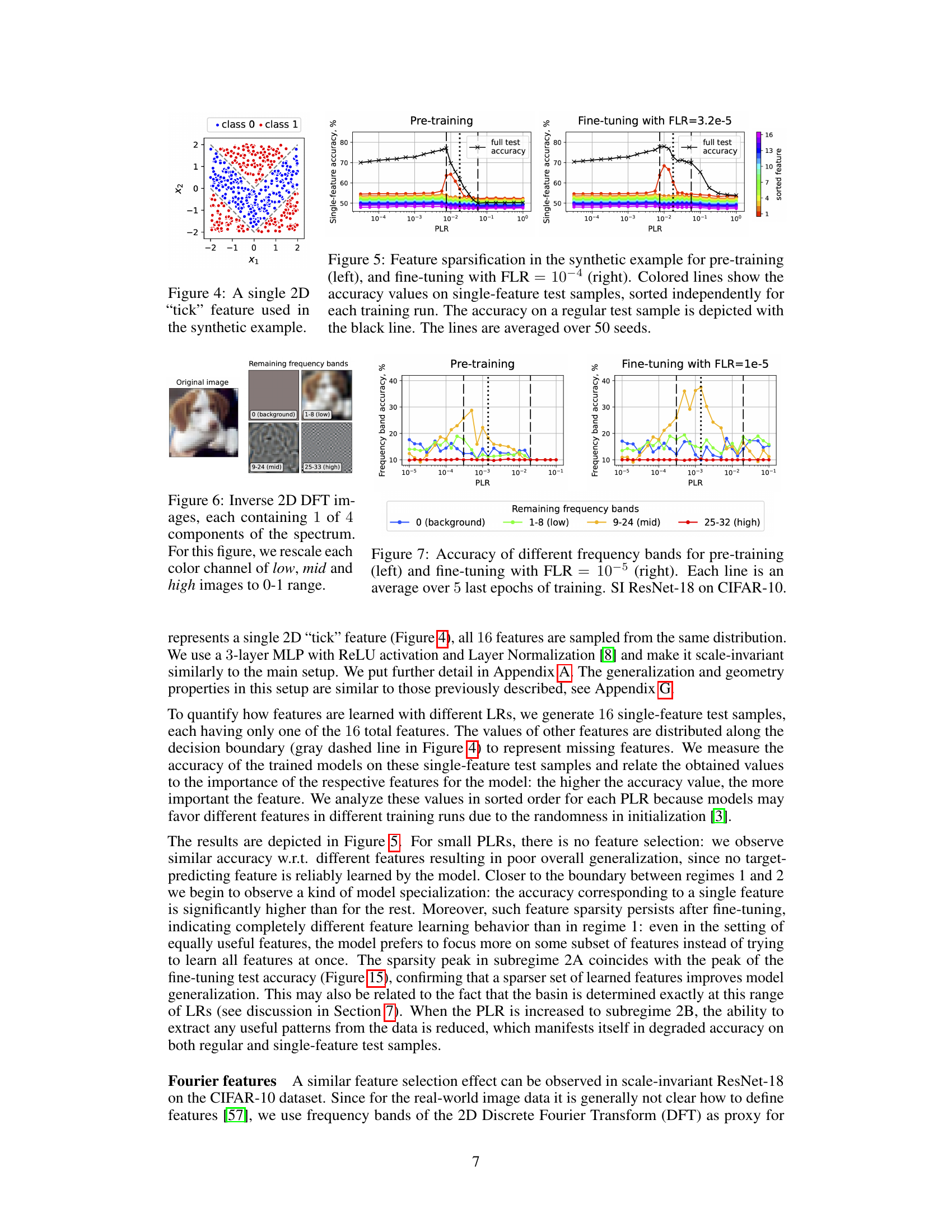
🔼 The figure shows four images. The leftmost image is the original image. The remaining three images are obtained via inverse 2D DFT of the original image, each containing only one of the four frequency bands: 0 (background), 1-8 (low), 9-24 (mid), and 25-32 (high). Each color channel of the low, mid, and high images are rescaled to the range [0,1].
read the caption
Figure 6: Inverse 2D DFT images, each containing 1 of 4 components of the spectrum. For this figure, we rescale each color channel of low, mid and high images to 0-1 range.
🔼 This figure shows the angular distance and the train/test error barriers between three solutions for each PLR: SWA of 5 networks and the points obtained after fine-tuning with the lowest and the highest considered FLRs. It provides a visual representation of the loss landscape geometry to help understand the effects of different initial learning rates.
read the caption
Figure 3: Geometry between the points fine-tuned with the smallest and the largest FLRs and SWA. SI ResNet-18 on CIFAR-10.

🔼 This figure shows the test accuracy results for fine-tuning and SWA (Stochastic Weight Averaging) methods applied on a scale-invariant ResNet-18 model trained on the CIFAR-10 dataset. The left panel displays fine-tuning results, while the right shows SWA results. The black line represents the test accuracy achieved after the pre-training phase with different pre-training learning rates (PLRs). The colored lines show the test accuracy after fine-tuning (left) or SWA (right) with varying fine-tuning learning rates (FLRs) or number of models averaged, respectively. The dashed lines indicate the boundaries separating the three main training regimes, and the dotted line further divides the second regime into two subregimes (2A and 2B). The figure highlights the optimal initial learning rate range for achieving the best generalization performance after fine-tuning or SWA.
read the caption
Figure 2: Test accuracy of the fine-tuned (left) and SWA (right) solutions for SI ResNet-18 on CIFAR-10. Test accuracy after pre-training is depicted with the black line. Dashed lines denote boundaries between the pre-training regimes, dotted line divides the second regime into two subregimes.

🔼 This figure shows the results of applying the inverse 2D Discrete Fourier Transform (DFT) to an image after masking specific frequency bands. The top row displays the reconstructed images using different frequency components (0 representing the constant background, 1-8 representing low frequencies, 9-24 representing mid frequencies, and 25-32 representing high frequencies). The bottom row shows the corresponding masked spectra (the logarithm of the amplitude values summed over the three color channels). This visualization helps to understand how different frequency components contribute to the overall image content.
read the caption
Figure 9: Inverse 2D DFT images (top) and corresponding masked spectra (bottom). When visualizing the low, mid, and high images, we scale each channel to the range 0–1. For the spectra, we plot the logarithm of the absolute values of the amplitudes (log |Y[k, l]|), summed over 3 color channels.

🔼 This figure shows the test accuracy results for fine-tuning and stochastic weight averaging (SWA) methods applied to a scale-invariant ResNet-18 model trained on the CIFAR-10 dataset. The x-axis represents the pre-training learning rate (PLR), and the y-axis represents the test accuracy. Different colored lines represent the test accuracy after fine-tuning with different fine-tuning learning rates (FLRs), while the black line shows the test accuracy after the pre-training stage. The dashed lines separate the three training regimes identified in the paper (convergence, chaotic equilibrium, and divergence). The dotted line further divides the second regime (chaotic equilibrium) into two sub-regimes (2A and 2B). This visualization helps to understand how different initial learning rates affect the final model performance and to identify the optimal range of initial learning rates (sub-regime 2A) for achieving best generalization after fine-tuning or SWA.
read the caption
Figure 2: Test accuracy of the fine-tuned (left) and SWA (right) solutions for SI ResNet-18 on CIFAR-10. Test accuracy after pre-training is depicted with the black line. Dashed lines denote boundaries between the pre-training regimes, dotted line divides the second regime into two subregimes.

🔼 This figure shows the test accuracy results for fine-tuning and Stochastic Weight Averaging (SWA) on a scale-invariant ResNet-18 model trained on CIFAR-10. The left panel displays the results of fine-tuning, while the right shows the SWA results. The black line represents the test accuracy achieved after the pre-training phase using different pre-training learning rates (PLRs). The colored lines represent the test accuracy after fine-tuning with different fine-tuning learning rates (FLRs) or after performing SWA. The dashed lines separate the three training regimes (convergence, chaotic equilibrium, and divergence), while the dotted line further subdivides the second regime into two subregimes (2A and 2B) based on the model’s performance. This figure is crucial in identifying the optimal initial learning rate range (subregime 2A) for achieving the best generalization after fine-tuning or SWA.
read the caption
Figure 2: Test accuracy of the fine-tuned (left) and SWA (right) solutions for SI ResNet-18 on CIFAR-10. Test accuracy after pre-training is depicted with the black line. Dashed lines denote boundaries between the pre-training regimes, dotted line divides the second regime into two subregimes.

🔼 This figure shows the test accuracy results for fine-tuned and SWA models on the CIFAR-10 dataset using a scale-invariant ResNet-18. The left panel shows the test accuracy after fine-tuning with different fine-tuning learning rates (FLRs), while the right panel displays the results using SWA with varying numbers of models. The black line represents the test accuracy after the initial pre-training phase with different pre-training learning rates (PLRs). Dashed lines separate the three training regimes (convergence, chaotic equilibrium, and divergence), while the dotted line further divides the second regime (chaotic equilibrium) into two subregimes (2A and 2B). The figure illustrates how the optimal PLR range (subregime 2A) significantly improves generalization compared to other PLR ranges.
read the caption
Figure 2: Test accuracy of the fine-tuned (left) and SWA (right) solutions for SI ResNet-18 on CIFAR-10. Test accuracy after pre-training is depicted with the black line. Dashed lines denote boundaries between the pre-training regimes, dotted line divides the second regime into two subregimes.

🔼 This figure shows the results of experiments aimed at determining the boundary between the first and second training regimes. The left panel shows the number of epochs required for the training process to converge when using different pre-training learning rates (PLRs). The right panel shows the test accuracy achieved after training to convergence with those same PLRs. Red dots indicate the test accuracy after training from scratch with a fixed LR value. The figure suggests that the optimal PLR for achieving high test accuracy lies just above the convergence threshold of the first training regime.
read the caption
Figure 11: Number of training epochs to convergence (left) and test accuracy (right) for different PLRs on the boundary between regimes 1 and 2. Red points are obtained after training to convergence from scratch with a fixed LR value (we run each experiment with three different seeds).
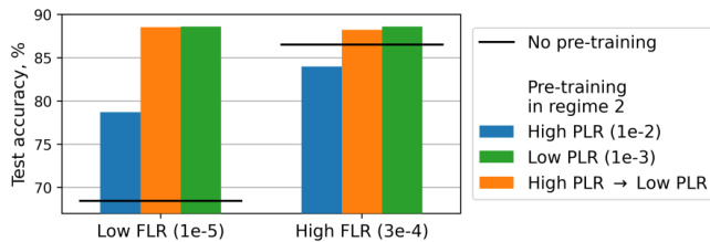
🔼 This figure compares test accuracy results from three different training scenarios: training from scratch with a low or high fine-tuning learning rate (FLR), training with a low or high pre-training learning rate (PLR) from subregime 2A, and training using a high PLR from subregime 2B followed by a low PLR from subregime 2A and then a given FLR. It shows that using a two-stage pre-training approach can improve the test accuracy compared to training from scratch or only using a single pre-training stage. This demonstrates the advantage of selecting initial learning rates above the convergence threshold but within a narrow range to reach optimal performance.
read the caption
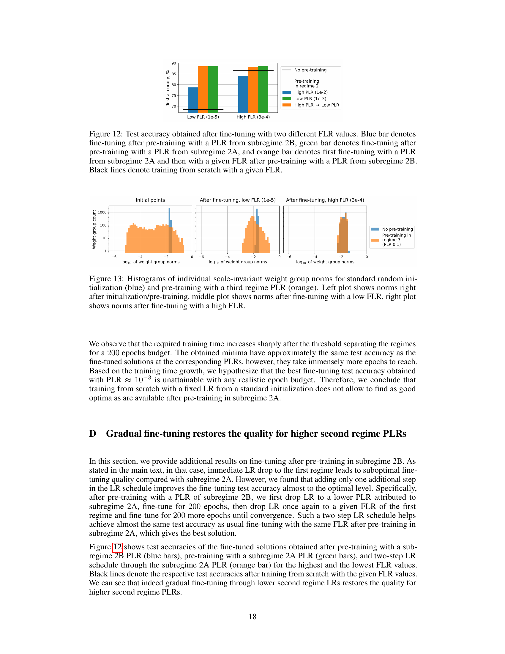
Figure 12: Test accuracy obtained after fine-tuning with two different FLR values. Blue bar denotes fine-tuning after pre-training with a PLR from subregime 2B, green bar denotes fine-tuning after pre-training with a PLR from subregime 2A, and orange bar denotes first fine-tuning with a PLR from subregime 2A and then with a given FLR after pre-training with a PLR from subregime 2B. Black lines denote training from scratch with a given FLR.

🔼 This figure displays the distribution of scale-invariant weight group norms at different training stages. The leftmost panel shows the initial distribution (standard random initialization vs. pre-training with a high learning rate in regime 3). The middle panel displays the distribution after fine-tuning with a low learning rate, and the rightmost panel shows the distribution after fine-tuning with a high learning rate. The figure highlights how the distribution of norms changes throughout the training process depending on the initial learning rate and the subsequent fine-tuning.
read the caption
Figure 13: Histograms of individual scale-invariant weight group norms for standard random initialization (blue) and pre-training with a third regime PLR (orange). Left plot shows norms right after initialization/pre-training, middle plot shows norms after fine-tuning with a low FLR, right plot shows norms after fine-tuning with a high FLR.

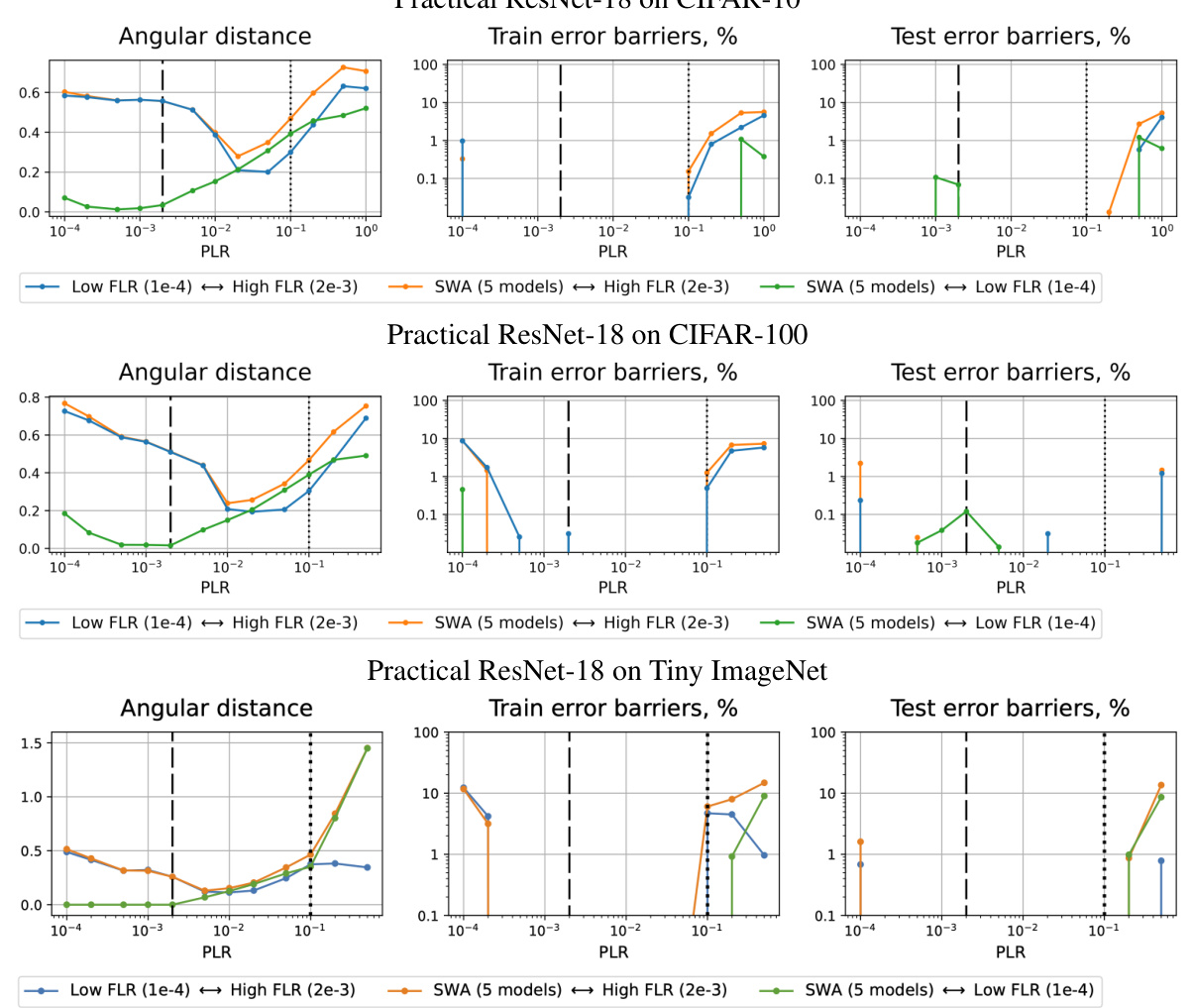
🔼 This figure shows the angular distance, train error barriers, and test error barriers between three solutions obtained with different fine-tuning learning rates (FLRs) for various pre-training learning rates (PLRs). The three solutions are: (1) fine-tuned with the lowest FLR, (2) fine-tuned with the highest FLR, and (3) obtained via Stochastic Weight Averaging (SWA) of five models. The figure visually represents the local geometry of the minima obtained from different pre-training conditions. The results are presented for different network architectures (SI ConvNet, SI ResNet-18) and datasets (CIFAR-10, CIFAR-100). The analysis shows how the initial learning rate impacts the landscape geometry, highlighting the key characteristics of minima reached using different learning rates. This provides additional insights into the relationship between model quality and the local geometry of the loss landscape, confirming findings from Figure 3 for different network architectures and datasets.
read the caption
Figure 14: Geometry between the points fine-tuned with the smallest and the largest FLRs and SWA. Results for other dataset-architecture pairs, similar to Figure 3.

🔼 This figure shows the test accuracy results for fine-tuning and Stochastic Weight Averaging (SWA) on a scale-invariant ResNet-18 model trained on CIFAR-10. The x-axis represents the pre-training learning rate (PLR), and the y-axis represents the test accuracy. The black line indicates the test accuracy after the pre-training stage. Different colored lines represent the results of fine-tuning with different fine-tuning learning rates (FLRs) and SWA with different numbers of models. The dashed lines indicate the boundaries between three different training regimes (convergence, chaotic equilibrium, divergence) based on the initial PLR. A dotted line further divides the second regime into two subregimes (2A and 2B). The figure illustrates how the optimal range for the initial PLR is within a narrow band in subregime 2A for both fine-tuning and SWA, leading to superior generalization performance.
read the caption
Figure 2: Test accuracy of the fine-tuned (left) and SWA (right) solutions for SI ResNet-18 on CIFAR-10. Test accuracy after pre-training is depicted with the black line. Dashed lines denote boundaries between the pre-training regimes, dotted line divides the second regime into two subregimes.

🔼 This figure shows the angular distances and error barriers between three different types of solutions obtained after pre-training with various initial learning rates (PLRs). The three solution types are: 1) fine-tuning with the smallest fine-tuning learning rate (FLR), 2) fine-tuning with the largest FLR, and 3) stochastic weight averaging (SWA) of 5 models. The x-axis represents the different PLRs used for pre-training, categorized into three regimes (convergence, chaotic equilibrium, and divergence) shown by dashed lines. The plot demonstrates the geometrical relationships between solutions obtained with different FLRs for each pre-training regime (PLR). This helps to understand how the choice of initial learning rate influences the final minima found and their interconnectivity in the loss landscape.
read the caption
Figure 3: Geometry between the points fine-tuned with the smallest and the largest FLRs and SWA. SI ResNet-18 on CIFAR-10.

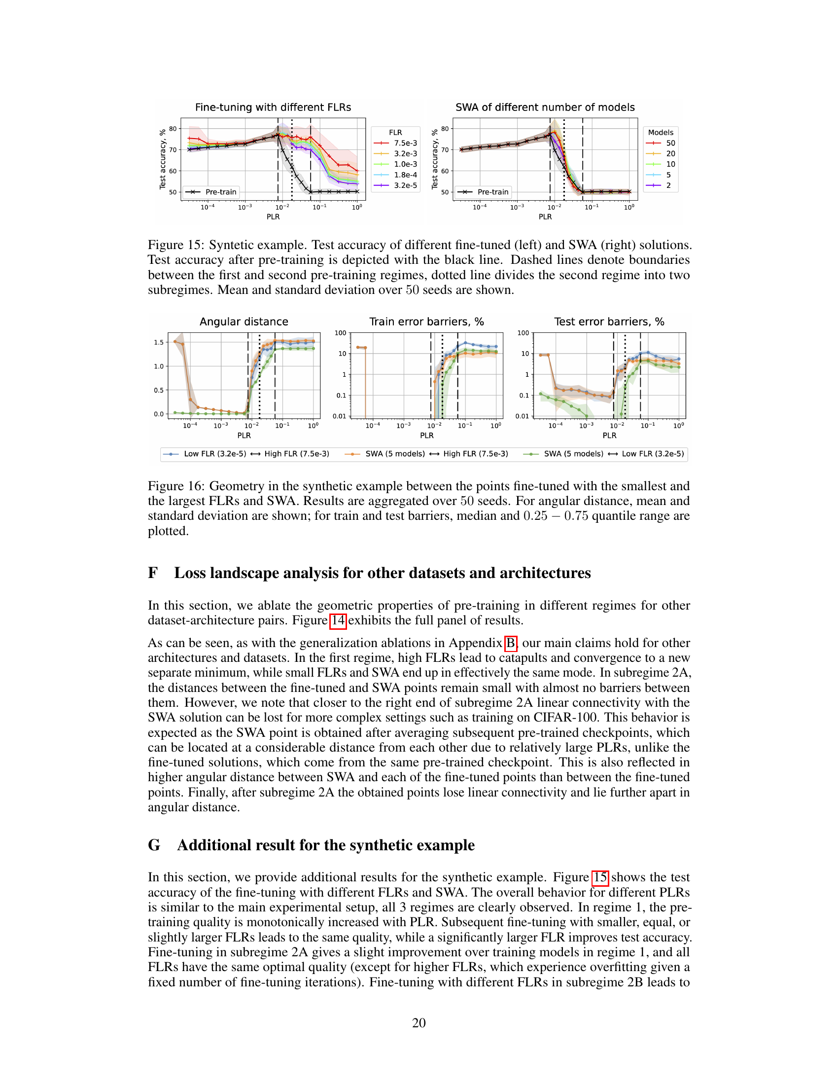
🔼 This figure shows the results of a synthetic experiment designed to study feature learning with different learning rates. The left panel shows the results of pre-training with different learning rates (PLRs), while the right panel shows the results of fine-tuning with a small learning rate (FLR) after pre-training with various PLRs. In both panels, the colored lines show the accuracy on test samples which contain only one feature at a time, while the black line shows the accuracy on regular test samples. The figure indicates that a narrow range of optimal PLRs leads to a model which focuses on learning only a sparse set of relevant features. This feature sparsity is preserved even after fine-tuning with a small FLR.
read the caption
Figure 5: Feature sparsification in the synthetic example for pre-training (left), and fine-tuning with FLR = 10-4 (right). Colored lines show the accuracy values on single-feature test samples, sorted independently for each training run. The accuracy on a regular test sample is depicted with the black line. The lines are averaged over 50 seeds.
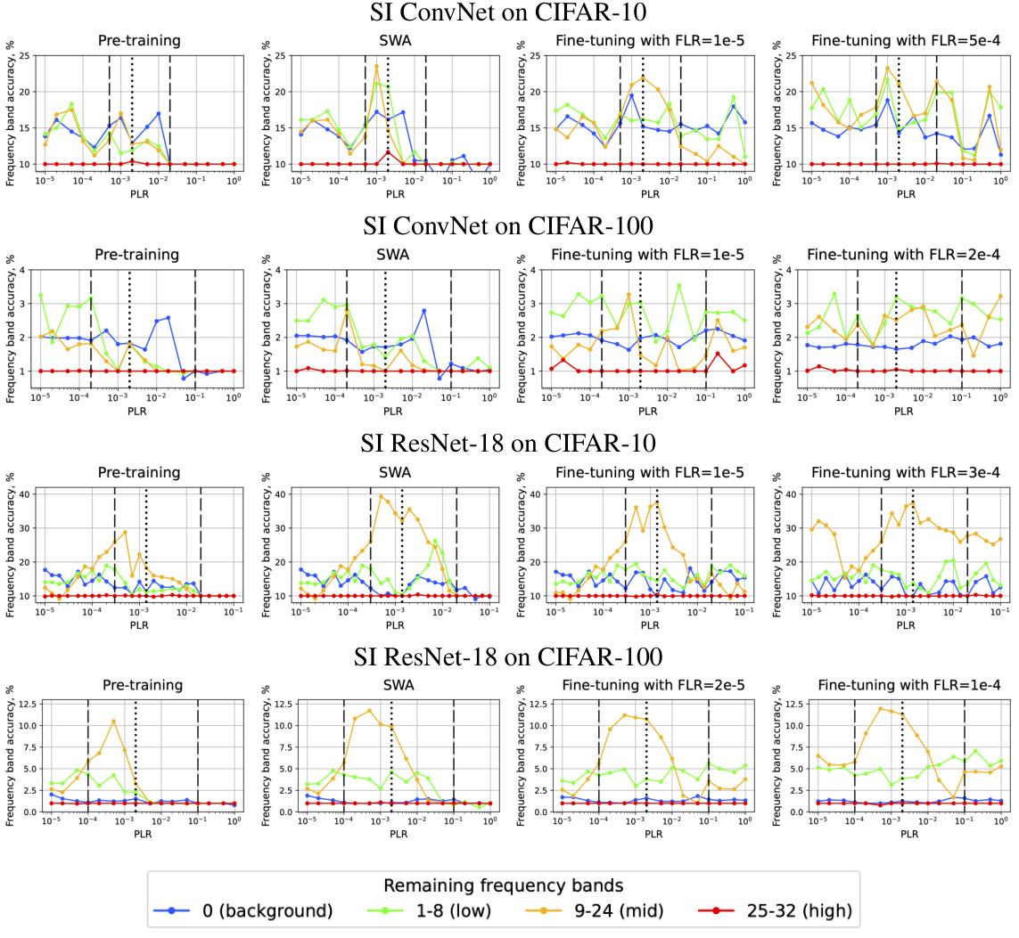
🔼 This figure compares the test accuracy of fine-tuned and SWA models across different pre-training learning rates (PLRs) for various model architectures (ConvNet and ResNet-18) and datasets (CIFAR-10 and CIFAR-100). It shows how the choice of the initial LR during pre-training affects the final test accuracy after fine-tuning with a small LR or weight averaging. The figure highlights the three training regimes identified in the paper (convergence, chaotic equilibrium, and divergence) and a crucial subregime (2A) within the chaotic equilibrium regime which yields optimal results. The black line represents the test accuracy after the initial pre-training phase, while colored lines show results after fine-tuning or SWA with different fine-tuning learning rates (FLRs).
read the caption
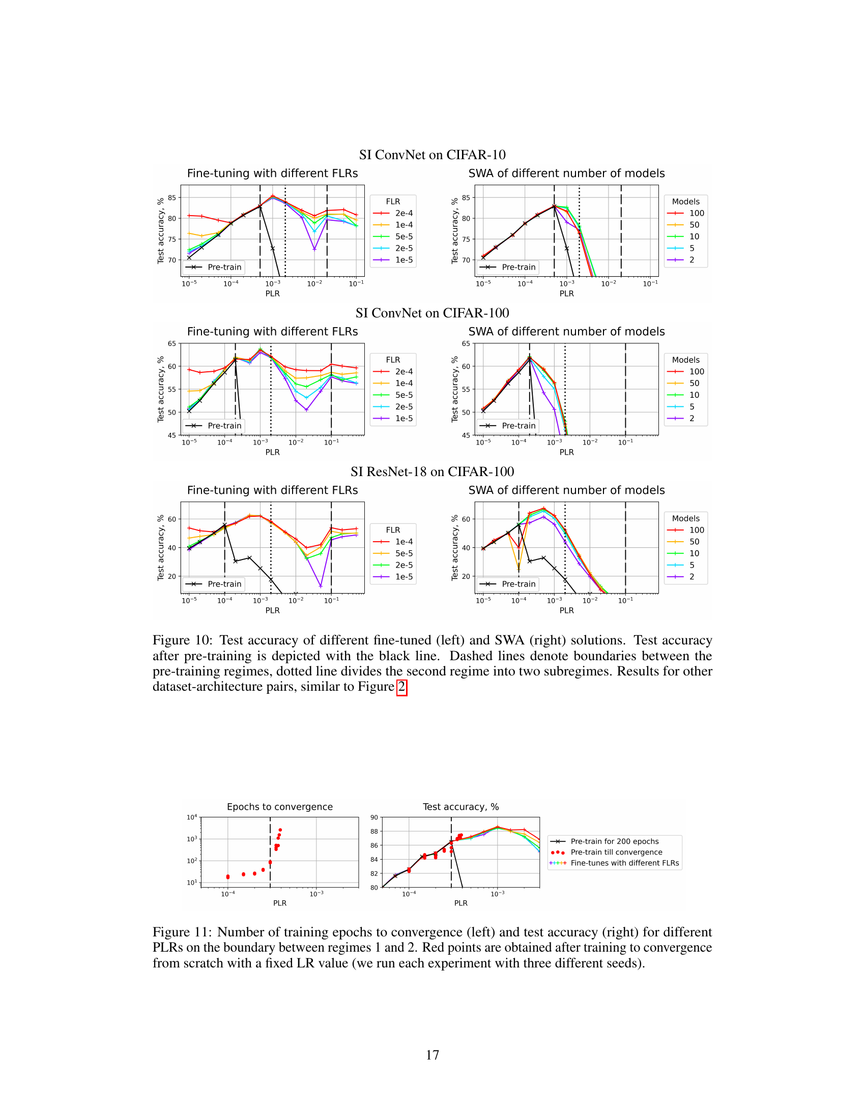
Figure 10: Test accuracy of different fine-tuned (left) and SWA (right) solutions. Test accuracy after pre-training is depicted with the black line. Dashed lines denote boundaries between the pre-training regimes, dotted line divides the second regime into two subregimes. Results for other dataset-architecture pairs, similar to Figure 2.

🔼 This figure shows the test accuracy results after fine-tuning with different fine-tuning learning rates (FLRs) and Stochastic Weight Averaging (SWA) with different numbers of models. The results are shown for a scale-invariant ResNet-18 model trained on the CIFAR-10 dataset. The black line represents the test accuracy after the pre-training phase using different pre-training learning rates (PLRs). The dashed lines separate the three training regimes identified in the paper (convergence, chaotic equilibrium, and divergence). The dotted line further subdivides the second regime into two subregimes (2A and 2B). This figure helps to illustrate the impact of choosing different PLRs on the final generalization performance after fine-tuning or SWA. The optimal range of PLRs that lead to the best generalization performance after fine-tuning or SWA is highlighted.
read the caption
Figure 2: Test accuracy of the fine-tuned (left) and SWA (right) solutions for SI ResNet-18 on CIFAR-10. Test accuracy after pre-training is depicted with the black line. Dashed lines denote boundaries between the pre-training regimes, dotted line divides the second regime into two subregimes.
🔼 This figure displays angular distances and error barriers between three solutions obtained after pre-training with various PLRs. The three solutions for each PLR are: 1) the solution obtained via fine-tuning with the smallest FLR (1e-5); 2) the solution obtained via fine-tuning with the largest FLR (3e-4); and 3) the solution obtained via SWA of 5 models. The plots show how these metrics vary with different PLRs across the three training regimes. This visualization helps to understand the local geometric properties of minima reached after training with different initial learning rates, providing insight into the optimization landscape and helping to explain why particular LRs lead to better generalization.
read the caption
Figure 3: Geometry between the points fine-tuned with the smallest and the largest FLRs and SWA. SI ResNet-18 on CIFAR-10.
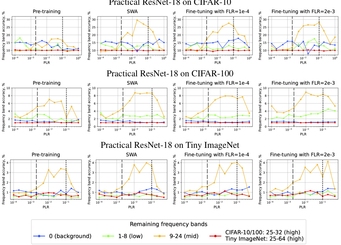
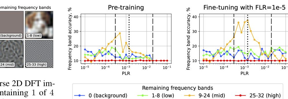
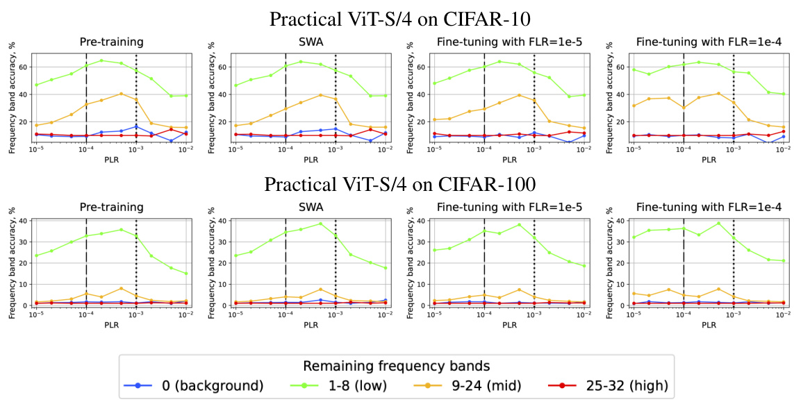
🔼 This figure shows the accuracy of different frequency bands for pre-training, SWA, and fine-tuning with low and high FLRs. The results are shown for SI ConvNet and SI ResNet-18 on CIFAR-10, CIFAR-100, and Tiny ImageNet datasets. Each column represents a different training approach, and each row represents a different dataset/architecture combination. The x-axis represents the pre-training learning rate (PLR), and the y-axis represents the accuracy of the corresponding frequency band.
read the caption
Figure 18. Accuracy of different frequency bands for pre-training (column 1), SWA (over 5 models; column 2), and fine-tuning with low FLR (column 3) and high FLR (column 4). SI ConvNet and SI ResNet-18 on CIFAR-10/CIFAR-100 and Tiny ImageNet.
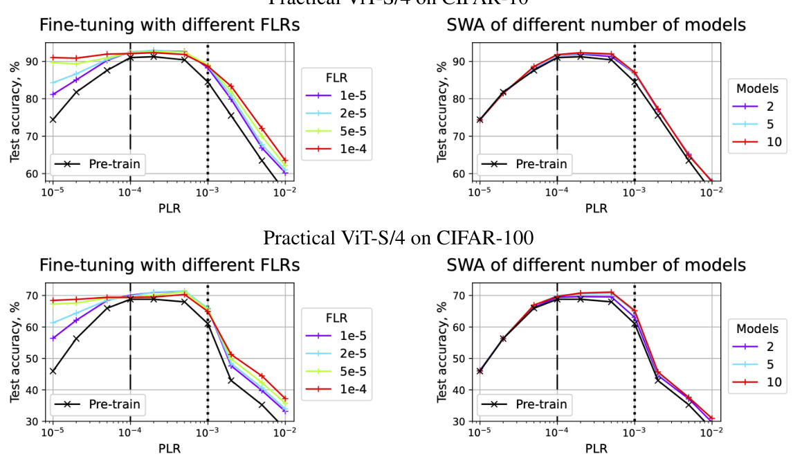
🔼 This figure shows the test accuracy results for fine-tuning and Stochastic Weight Averaging (SWA) on a scale-invariant ResNet-18 model trained on CIFAR-10 dataset. The x-axis represents the pre-training learning rate (PLR), and the y-axis shows the test accuracy. The black line indicates the test accuracy after the initial pre-training phase with different PLRs. Colored lines represent the test accuracy after further fine-tuning (left) with a small learning rate (FLR) or SWA (right) with different numbers of models. Dashed lines separate the three training regimes identified in the paper (convergence, chaotic equilibrium, and divergence), while the dotted line further divides the second regime into two subregimes (2A and 2B). The figure illustrates the impact of initial LR on the final model performance.
read the caption
Figure 2: Test accuracy of the fine-tuned (left) and SWA (right) solutions for SI ResNet-18 on CIFAR-10. Test accuracy after pre-training is depicted with the black line. Dashed lines denote boundaries between the pre-training regimes, dotted line divides the second regime into two subregimes.
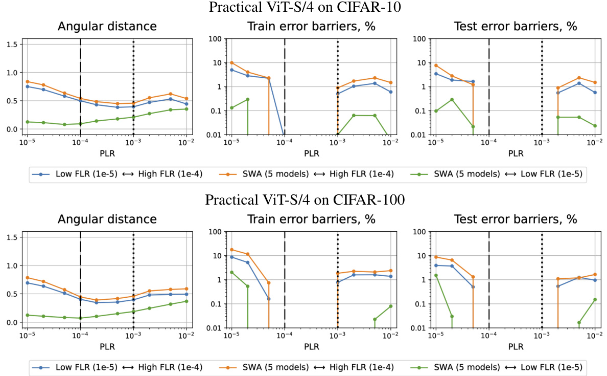
🔼 This figure visualizes the geometric relationships between different model solutions obtained through various training methods. Specifically, it shows the angular distance and error barriers (both training and test error) between three types of solutions for each pre-training learning rate (PLR): 1) Solutions obtained by fine-tuning with the smallest fine-tuning learning rate (FLR); 2) Solutions obtained by fine-tuning with the largest FLR; and 3) Stochastic Weight Averaging (SWA) of five models. The plot illustrates how the geometry of the loss landscape changes depending on the initial learning rate used for pre-training, providing insights into the optimization process and the quality of the solutions obtained. The SI ResNet-18 model was trained on CIFAR-10 dataset.
read the caption
Figure 3: Geometry between the points fine-tuned with the smallest and the largest FLRs and SWA. SI ResNet-18 on CIFAR-10.
🔼 This figure shows the test accuracy for various model architectures (SI ConvNet and SI ResNet-18) trained on different datasets (CIFAR-10 and CIFAR-100). It compares the results of fine-tuning with different final learning rates (FLRs) and stochastic weight averaging (SWA) after pre-training with different pre-training learning rates (PLRs). The black line represents the test accuracy after the pre-training stage. Dashed lines separate the three training regimes (convergence, chaotic equilibrium, divergence), and the dotted line further subdivides the second regime (chaotic equilibrium) into two subregimes (2A and 2B). The plot illustrates how the optimal range of initial learning rates for obtaining high generalization performance after fine-tuning or SWA varies depending on the model architecture and dataset.
read the caption
Figure 10: Test accuracy of different fine-tuned (left) and SWA (right) solutions. Test accuracy after pre-training is depicted with the black line. Dashed lines denote boundaries between the pre-training regimes, dotted line divides the second regime into two subregimes. Results for other dataset-architecture pairs, similar to Figure 2.
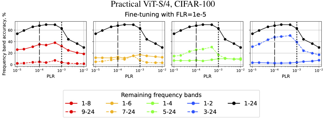
🔼 This figure shows how the accuracy of different frequency bands changes when varying the boundary between low and mid-frequencies for fine-tuning with a small learning rate (FLR) in the practical setting using Vision Transformer (ViT). The x-axis represents the pre-training learning rate (PLR), and the y-axis represents the accuracy for different frequency ranges. The different colored lines show the accuracy for different frequency bands. The figure demonstrates how the choice of pre-training learning rate (PLR) affects the learned features, and that there is an optimal range for generalization.
read the caption
Figure 25: Practical setting on ViT. Accuracy of different frequency bands when varying the boundary between low and mid-frequencies for fine-tuning with small FLR.

🔼 This figure shows the relationship between sharpness and test error for fine-tuned solutions obtained after pre-training with different learning rates. Each point represents a fine-tuned model with the same pre-training point but different fine-tuning learning rates. The color of the point indicates the pre-training learning rate, ranging from low (purple) to high (red). Black points represent pre-trained models without fine-tuning. The figure demonstrates that while there’s a general trend suggesting that models with lower sharpness have lower test error, the relationship is not straightforward and the sharpness is not a reliable indicator of generalization in this particular setting.
read the caption
Figure 26: Scatter plot of sharpness vs. test error for the fine-tuned solutions at the same level of the training loss. Groups of points of the same color represent fine-tuned solutions with different FLRs but with the same pre-trained point. Different colors denote different PLRs of the second regime: from low (purple) to high (red). Black dots correspond to the pre-trained points of the first regime, replicating the results of Kodryan et al. [35]. SI ResNet-18 on CIFAR-10.
Full paper#

