TL;DR#
Current dynamic novel view synthesis methods struggle with high computational costs, especially when dealing with dynamic motions and limited computing resources. Existing techniques often rely on implicit representations or dense data, which hinders real-time performance and scalability. This limitation becomes particularly apparent when processing dynamic scenes for videos, where the processing needs to handle temporal information. Existing 3D Gaussian Splatting methods are effective for static scenes, but extending them to handle dynamic scenes while maintaining efficiency has been a challenge.
Ex4DGS addresses these challenges using a novel keyframe interpolation approach. By separating static and dynamic Gaussians and sampling them sparsely at keyframes, it reduces computational cost while maintaining continuous motion representation. The progressive training scheme and point-backtracking technique further enhance convergence and quality. The method achieves fast and high-quality rendering, outperforming existing methods on benchmark datasets. This highlights the efficiency and scalability of Ex4DGS for real-world applications.
Key Takeaways#
Why does it matter?#
This paper is crucial for researchers in computer graphics and computer vision because it significantly advances the state-of-the-art in dynamic novel view synthesis. By introducing Explicit 4D Gaussian Splatting (Ex4DGS), it offers a novel approach to handle the challenges of dynamic scenes with improved speed and efficiency. Its focus on explicit representations, keyframe interpolation, and progressive training provides new avenues for high-quality and real-time rendering, making it highly relevant to the current research trends focused on efficient and scalable view synthesis techniques for dynamic content. The success of the method on real-world datasets further solidifies its impact and potential for broader applications.
Visual Insights#

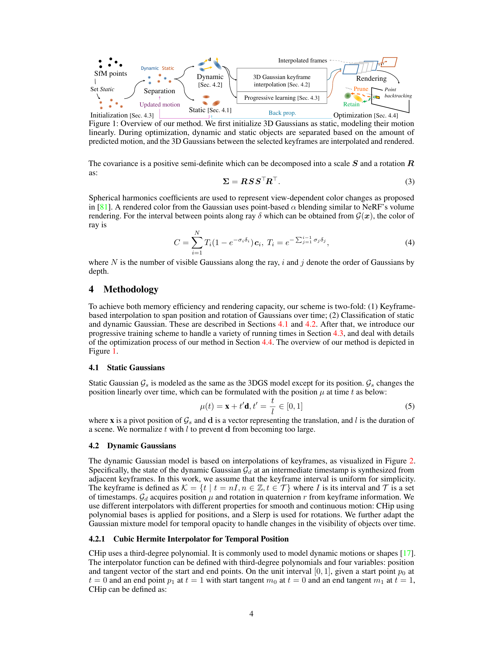
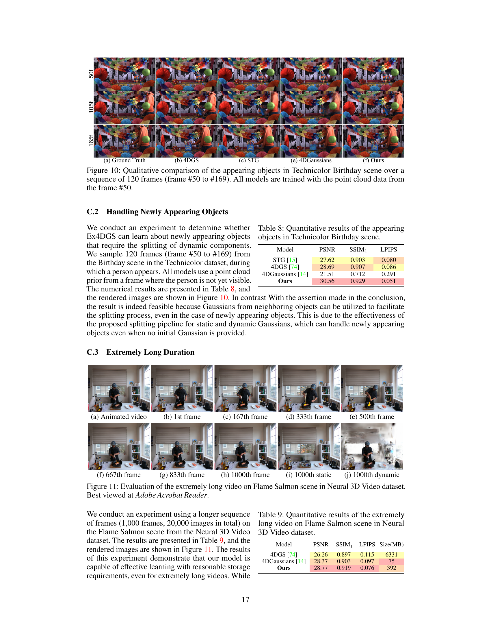
🔼 This figure illustrates the overall process of the proposed Explicit 4D Gaussian Splatting (Ex4DGS) method. It starts by initializing 3D Gaussians as static, whose motion is modeled linearly. During the optimization process, the algorithm separates dynamic and static objects based on their motion. The dynamic Gaussians’ position and rotation are interpolated between keyframes to achieve temporally continuous motion, while static Gaussians maintain linear motion. Finally, a point backtracking technique is used to refine the results by identifying and pruning erroneous Gaussians. The interpolated dynamic Gaussians are then rendered to generate the final output.
read the caption
Figure 1: Overview of our method. We first initialize 3D Gaussians as static, modeling their motion linearly. During optimization, dynamic and static objects are separated based on the amount of predicted motion, and the 3D Gaussians between the selected keyframes are interpolated and rendered.
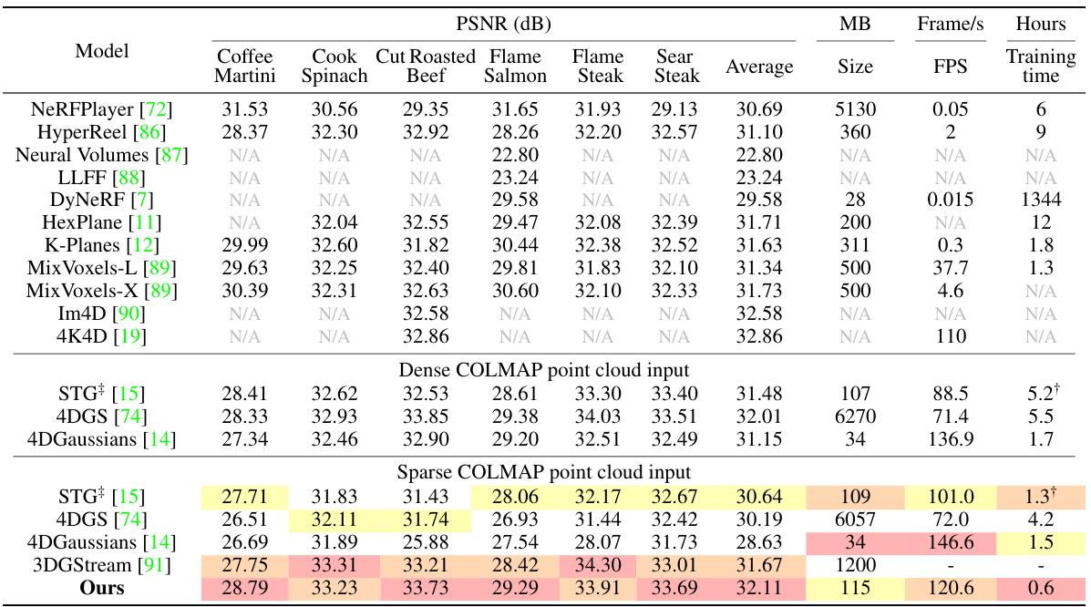
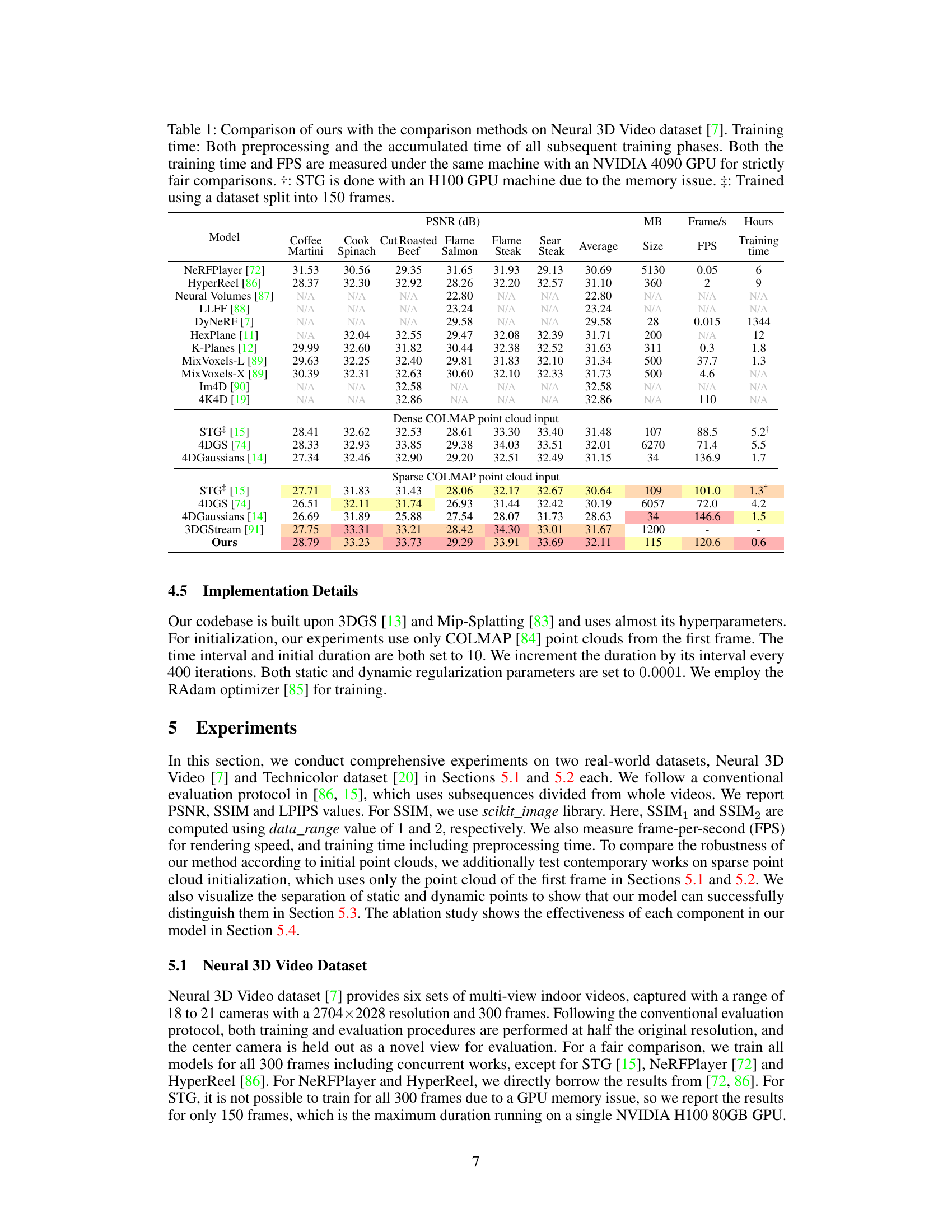
🔼 This table compares the proposed Explicit 4D Gaussian Splatting (Ex4DGS) method with other state-of-the-art dynamic novel view synthesis methods on the Neural 3D Video dataset. The comparison includes PSNR, SSIM, and LPIPS metrics, as well as training time, model size, and frames per second (FPS). The table is divided into sections based on whether dense or sparse COLMAP point cloud input was used, highlighting the robustness of Ex4DGS to different data conditions. Footnotes clarify specific experimental details.
read the caption
Table 1: Comparison of ours with the comparison methods on Neural 3D Video dataset [7]. Training time: Both preprocessing and the accumulated time of all subsequent training phases. Both the training time and FPS are measured under the same machine with an NVIDIA 4090 GPU for strictly fair comparisons. †: STG is done with an H100 GPU machine due to the memory issue. ‡: Trained using a dataset split into 150 frames.
In-depth insights#
Explicit 4DGS#
The concept of “Explicit 4DGS” suggests a significant advancement in 4D Gaussian splatting, moving beyond implicit representations to achieve enhanced efficiency and scalability. This approach likely involves explicitly representing the temporal dimension by directly storing keyframes for dynamic Gaussian parameters (position, rotation, and opacity), rather than relying on implicit neural networks to infer them. This explicit representation is key to reducing computational costs and enabling fast rendering speeds. The separation of static and dynamic Gaussians during training and the use of interpolation techniques between keyframes would further optimize processing. A progressive training scheme, starting with short time intervals and gradually increasing them, likely improves convergence, especially beneficial for handling sparse point clouds in real-world scenarios. The addition of a point-backtracking technique helps to address cumulative errors and improves the model’s robustness. Overall, “Explicit 4DGS” promises a more efficient and accurate approach to dynamic scene representation, potentially enabling real-time view synthesis applications.
Progressive Training#
Progressive training, as discussed in the context of the research paper, is a crucial technique for enhancing the model’s efficiency and robustness, particularly in scenarios involving dynamic scenes and sparse data. The core idea is to gradually increase the complexity of the training process, starting with short time durations and limited data points and progressively extending the duration and incorporating more data over time. This approach helps the model to avoid falling into local minima during the training phase and allows it to learn more effectively from sparse data. By gradually increasing the temporal and spatial complexity, progressive training allows for better generalization, resulting in a more robust and accurate model. The method is particularly beneficial when dealing with dynamic scenes, where sudden changes in object appearances or movements might disrupt the training. Starting with short clips and gradually extending the length allows the model to effectively learn and adapt to the dynamic changes. Furthermore, the progressive training scheme is designed to be computationally efficient, making it suitable for real-world applications where memory and computational resources are limited. It also improves the overall efficiency of the system by preventing the model from being overwhelmed by the initial complexity of the scene. The point-backtracking technique further enhances this strategy by removing erroneous Gaussians during the training process.
Dynamic Point Sep.#
The heading ‘Dynamic Point Sep.’ suggests a method within the research paper for separating or classifying points in a dataset based on their dynamic properties. This is likely crucial for efficiently handling dynamic scenes in applications like video processing or 3D modeling, where some elements are static while others move. The core idea is to distinguish between static and dynamic components of a scene automatically, potentially using motion-based triggers or other criteria. The approach enables selective processing, optimizing computational efficiency by reducing the amount of data requiring temporal modeling. By isolating dynamic points, the algorithm might only need to store and process additional temporal information for the moving parts, simplifying the representation and rendering. This separation technique is expected to improve performance, both in terms of training speed and rendering speed, compared to approaches that handle all points as equally dynamic, as it reduces computational complexity and memory usage. The effectiveness of dynamic point separation likely hinges on the accuracy and robustness of its underlying motion detection or classification mechanisms.
Keyframe Interpol.#
The concept of ‘Keyframe Interpolation’ in the context of dynamic 3D Gaussian splatting is crucial for efficient and high-quality video rendering. Instead of storing data for every frame, this technique strategically selects keyframes and interpolates the position, rotation, and opacity of Gaussians to reconstruct intermediate frames. This significantly reduces computational cost and memory usage while maintaining temporal coherence. Cubic Hermite splines are used for interpolating positions, enabling smooth transitions, while spherical linear interpolation (Slerp) handles rotations, accounting for the non-linear nature of angles. A simplified Gaussian mixture model is employed for opacity changes over time, addressing object appearance and disappearance. The selection of appropriate interpolation techniques and the implementation of keyframes are key to striking a balance between accuracy and computational efficiency. Sparse keyframe selection further enhances performance, and methods for distinguishing static and dynamic objects allow focusing interpolation efforts primarily where needed.
Future Work#
Future work for Explicit 4D Gaussian Splatting (Ex4DGS) could involve several key areas. Improving handling of occlusions and newly appearing objects is crucial. The current method struggles when objects suddenly appear or disappear; more sophisticated temporal modeling, perhaps leveraging prediction techniques or more robust mixture models for opacity, could be beneficial. Extending the approach to handle more complex motions is another promising direction. While Ex4DGS handles linear and smooth transitions well, more intricate movements might require adapting interpolation techniques or incorporating physics-based priors. Addressing the computational cost for extremely long videos remains important. While the progressive training scheme helps, exploring further optimizations, perhaps involving efficient data structures or hierarchical representations, is necessary to ensure scalability for real-world applications. Finally, exploring the integration of semantic information would enhance the system, allowing for more intelligent separation of dynamic and static elements and resulting in improved rendering quality and reduced computational load.
More visual insights#
More on figures

🔼 The figure demonstrates the effectiveness of the proposed keyframe interpolation method. It shows three subfigures. (a) shows a rendered image at a specific time (t). (b) illustrates the interpolated dynamic points that have been calculated based on the keyframes and their translations and rotations. (c) shows the rendered image at a subsequent time (t+I). The interpolated dynamic points smoothly transition between keyframes, resulting in a visually consistent and temporally coherent representation of dynamic motions. This visual representation strongly supports the method’s ability to efficiently model dynamic motions.
read the caption
Figure 2: Effectiveness of our keyframe interpolation.

🔼 This figure compares three different approaches to modeling temporal opacity: a single Gaussian, Gaussian mixtures, and the proposed method. The x-axis represents time, and the y-axis represents opacity (σt). The red line shows the actual opacity change over time, while the blue line shows the estimated opacity. (a) shows the limitations of using a single Gaussian to model complex opacity changes. (b) demonstrates the use of Gaussian mixtures to handle more complex changes. (c) illustrates how the authors’ proposed method addresses the limitations of the previous approaches and achieves better results.
read the caption
Figure 3: Comparison between the single Gaussian, Gaussian mixture, and our model for temporal opacity modeling.
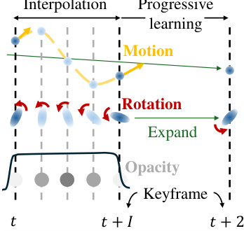
🔼 This figure illustrates the overall pipeline of the proposed Explicit 4D Gaussian Splatting (Ex4DGS) method. It starts by initializing all Gaussian points as static, assuming linear motion. During optimization, it dynamically separates static and dynamic objects based on predicted motion. The dynamic Gaussians’ positions and rotations are then interpolated between keyframes, resulting in smooth and continuous motion representation. The final step involves rendering the interpolated Gaussians to generate the output frames. The figure highlights the key stages: initialization, static/dynamic separation, progressive learning, point backtracking, and rendering.
read the caption
Figure 1: Overview of our method. We first initialize 3D Gaussians as static, modeling their motion linearly. During optimization, dynamic and static objects are separated based on the amount of predicted motion, and the 3D Gaussians between the selected keyframes are interpolated and rendered.

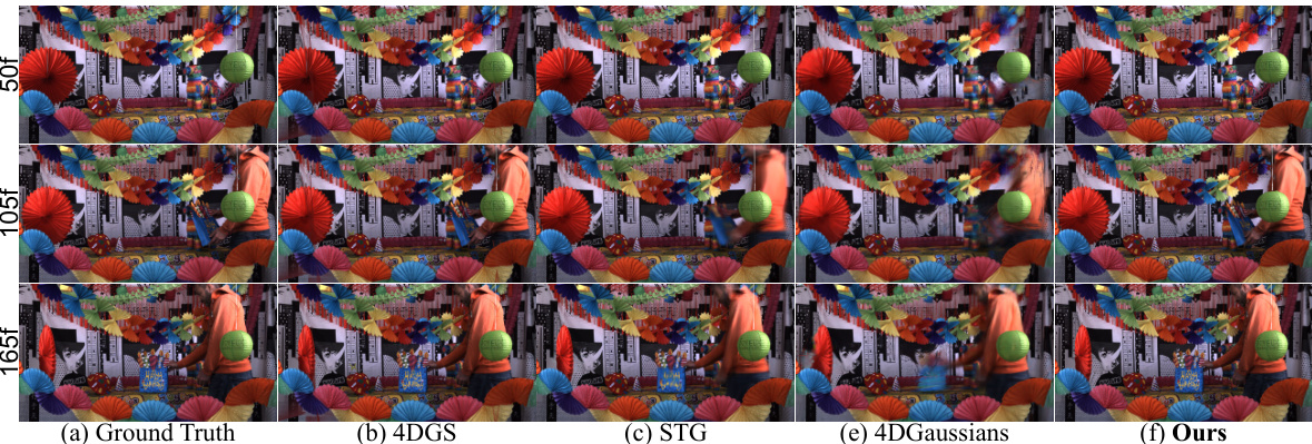
🔼 This figure compares the visual results of Ex4DGS against other state-of-the-art dynamic Gaussian splatting methods on the Neural 3D Video dataset. It shows example renderings from several scenes, allowing a visual comparison of rendering quality across different models. The goal is to highlight Ex4DGS’s superior performance in generating high-quality images, even in challenging scenarios with dynamic motion.
read the caption
Figure 5: Comparison of our Ex4DGS with other the state-of-the-art dynamic Gaussian splatting methods on Neural 3D Video [7] dataset.

🔼 This figure visualizes the separation of static and dynamic points achieved by the proposed method, Ex4DGS. It demonstrates the model’s ability to distinguish between static and dynamic components within a scene. The images show the ground truth, rendered static points only, rendered dynamic points only, and the combination of both. The examples are taken from the Neural 3D Video and Technicolor datasets, highlighting the method’s effectiveness across different scenes and datasets.
read the caption
Figure 6: Visualization of our static and dynamic point separation on Coffee Martini, Flame Steak and Fabien scene in Neural 3D Video [7] and Technicolor [20] datasets.

🔼 This figure compares the results of handling color changes in a video scene with two different methods. (b) shows the result when only color changes are considered, without differentiating between static and dynamic objects. The results show that static points cannot effectively handle these changes. (c) shows the result with the complete model where dynamic objects are treated differently, leading to better visual quality.
read the caption
Figure 7: Comparison between (b) handling color changes without dynamic points and (c) our complete model.

🔼 This figure compares the performance of different dynamic view synthesis methods (4DGS, 4D Gaussians, STG, and the proposed Ex4DGS) on a sequence of frames from the Technicolor Train scene where objects are repeatedly occluded. The models are all trained using only point cloud data from the initial frame (#170). The figure aims to demonstrate the ability of each method to handle occlusions and maintain rendering quality. The highlighted areas show the main area of comparison and focus.
read the caption
Figure 9: Qualitative comparison of the repeatedly occluded objects in the Technicolor Train scene over a sequence of 100 frames (frame #170 to #269). All models are trained with the point cloud data from the frame #170.
🔼 This figure illustrates the workflow of the proposed Explicit 4D Gaussian Splatting (Ex4DGS) method. It starts by initializing 3D Gaussians as static, assuming linear motion. During optimization, the method distinguishes between static and dynamic objects based on the predicted motion. Dynamic Gaussians are then interpolated between keyframes to create temporally continuous motion and finally rendered.
read the caption
Figure 1: Overview of our method. We first initialize 3D Gaussians as static, modeling their motion linearly. During optimization, dynamic and static objects are separated based on the amount of predicted motion, and the 3D Gaussians between the selected keyframes are interpolated and rendered.
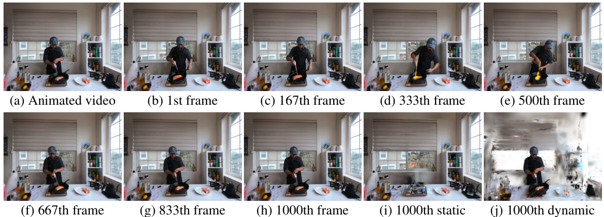
🔼 This figure visualizes the results of an experiment using an extremely long video sequence (1000 frames, 20000 images) on the Flame Salmon scene from the Neural 3D Video dataset. It showcases the rendering quality and robustness of the Ex4DGS model over an extended duration and illustrates how well it handles long sequences, maintaining high quality even with many frames. The figure compares the rendered results with the actual video frames.
read the caption
Figure 11: Evaluation of the extremely long video on Flame Salmon scene in Neural 3D Video dataset. Best viewed at Adobe Acrobat Reader.
More on tables
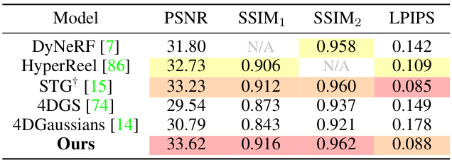
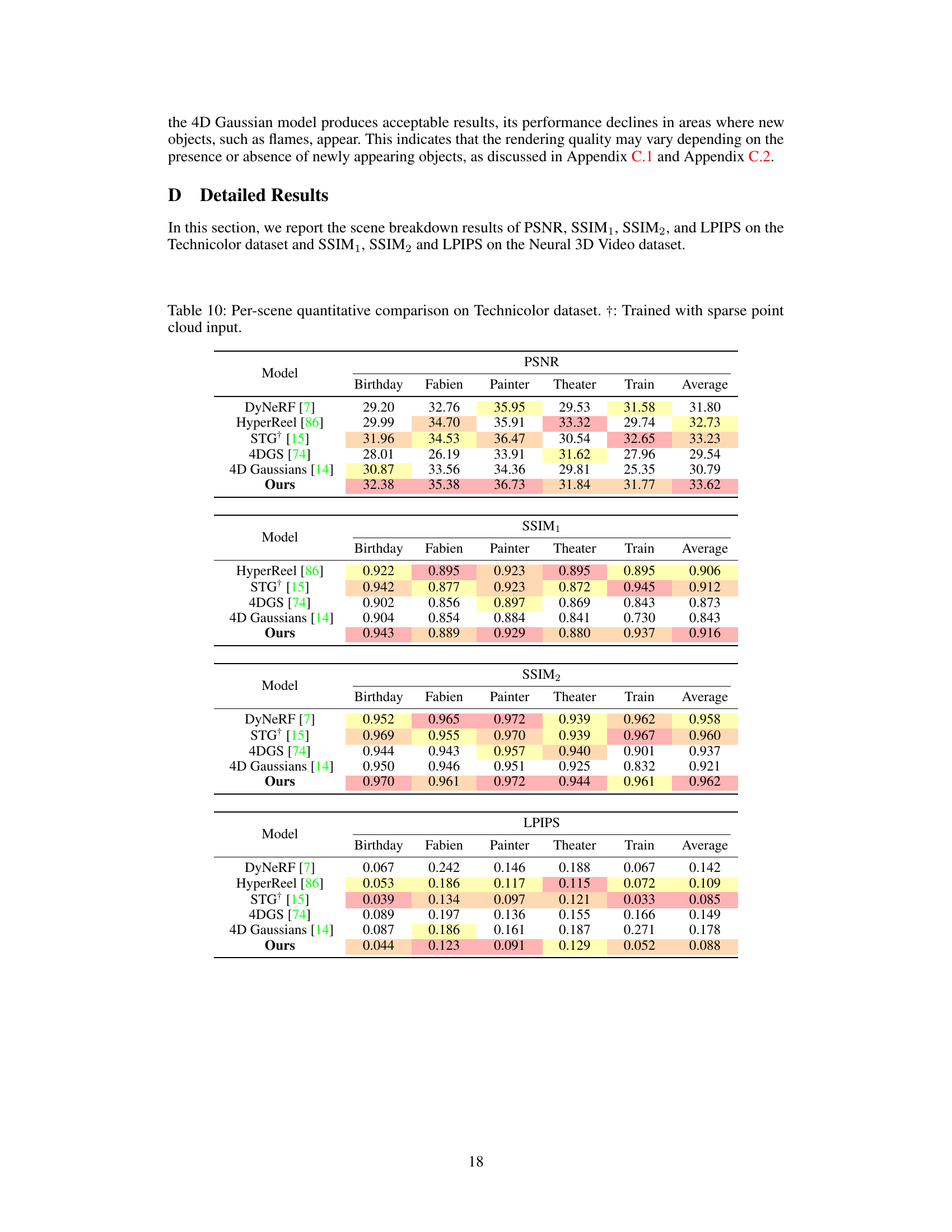
🔼 This table compares the performance of different novel view synthesis methods on the Technicolor dataset. The metrics used are PSNR, SSIM1, SSIM2, and LPIPS. The results are shown for both scenarios: using dense and sparse COLMAP point cloud inputs. The table highlights that the proposed Ex4DGS method achieves high performance even with sparse input.
read the caption
Table 2: Comparison results on the Technicolor dataset [20]. †: Trained with sparse point cloud input.
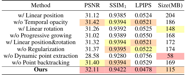
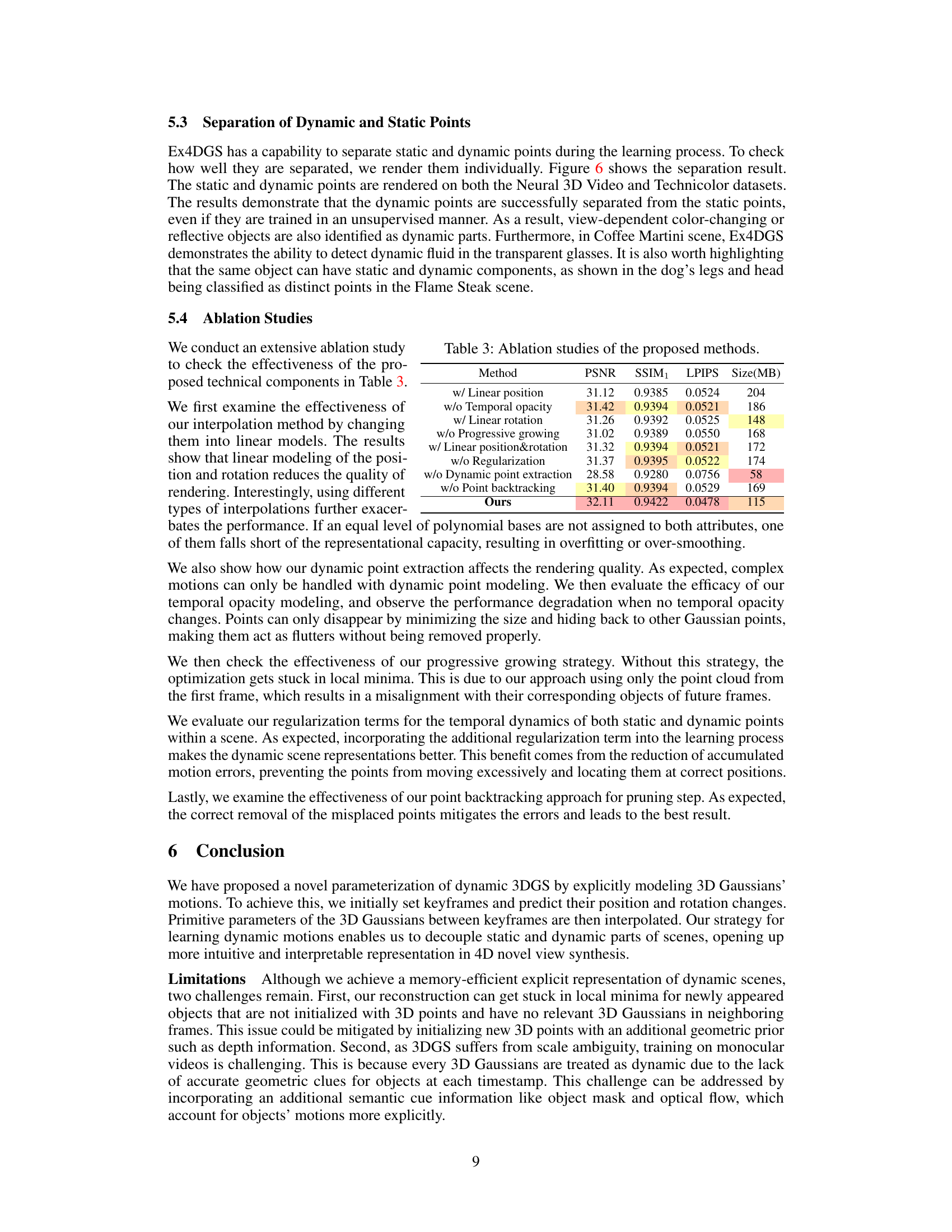
🔼 This table presents the ablation study of the proposed method, Explicit 4D Gaussian Splatting (Ex4DGS). It shows the impact of different components of the Ex4DGS model on its performance, as measured by PSNR, SSIM1, LPIPS, and model size (in MB). The ablation study systematically removes or replaces different components such as the interpolation method, the temporal opacity, and the progressive training scheme to evaluate their contribution to the overall performance.
read the caption
Table 3: Ablation studies of the proposed methods.

🔼 This table compares the performance of the 3DGS model (without handling color changes) against Ex4DGS (our complete model) on the Coffee Martini scene of the Neural 3D video dataset. It shows that Ex4DGS significantly outperforms the baseline 3DGS model in terms of PSNR, SSIM1, and LPIPS, highlighting the importance of incorporating dynamic points to accurately handle changes in color and appearance.
read the caption
Table 4: Comparison results between without handling color changes and our complete model.

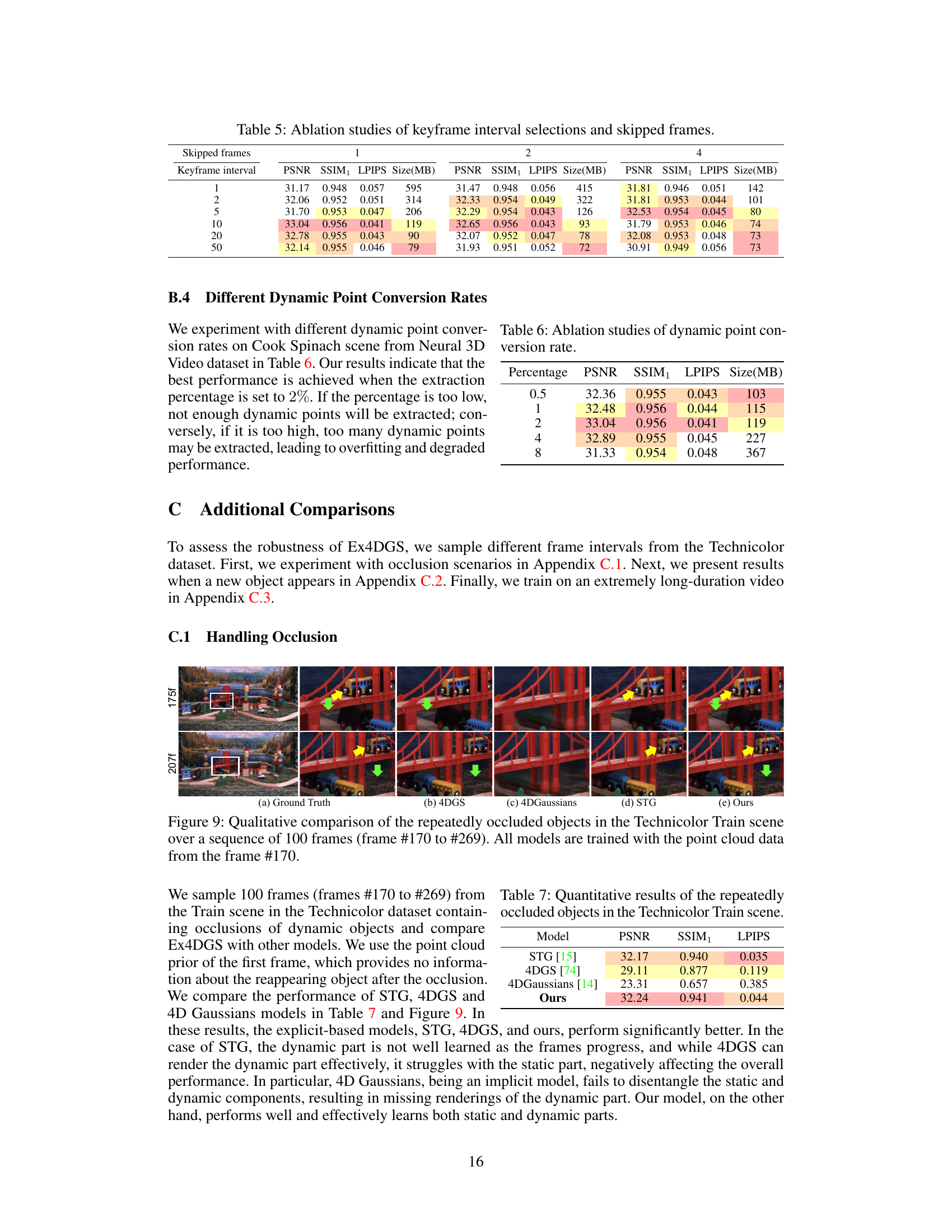
🔼 This table presents the ablation study results on the effects of different keyframe intervals and motion magnitudes on the performance of the proposed method. The experiment was conducted on the Cook Spinach scene from the Neural 3D Video dataset. The table shows how PSNR, SSIM1, LPIPS, and model size (in MB) vary across different combinations of skipped frames (simulating various motion speeds) and keyframe intervals.
read the caption
Table 5: Ablation studies of keyframe interval selections and skipped frames.

🔼 This table presents the ablation study results on the dynamic point conversion rate. It shows the PSNR, SSIM1, LPIPS, and model size (in MB) achieved using different percentages of dynamic points extracted during training. The results indicate an optimal balance between the number of dynamic points and model performance; using too few or too many points can lead to suboptimal results.
read the caption
Table 6: Ablation studies of dynamic point conversion rate.

🔼 This table presents a quantitative comparison of different novel view synthesis methods on the repeatedly occluded objects in the Technicolor Train scene. The metrics used for comparison are PSNR, SSIM1, and LPIPS. The results highlight the performance of each model in handling occlusions, showing how well they maintain image quality when objects are partially or completely hidden.
read the caption
Table 7: Quantitative results of the repeatedly occluded objects in the Technicolor Train scene.

🔼 This table presents a quantitative comparison of different methods for handling newly appearing objects in the Technicolor Birthday scene. The metrics used for comparison are PSNR, SSIM1, and LPIPS. The results show that the proposed method (Ours) outperforms the other methods, achieving significantly higher PSNR and SSIM1 values while having a much lower LPIPS value, which indicates better visual quality.
read the caption
Table 8: Quantitative results of the appearing objects in Technicolor Birthday scene.

🔼 This table presents a quantitative comparison of different models on the Flame Salmon scene from the Neural 3D Video dataset using an extremely long video sequence (1000 frames). The metrics shown are PSNR, SSIM1, LPIPS, and model size. It highlights the performance of various methods when dealing with extended temporal durations.
read the caption
Table 9: Quantitative results of the extremely long video on Flame Salmon scene in Neural 3D Video dataset.

🔼 This table compares the proposed Ex4DGS model with several state-of-the-art dynamic Gaussian splatting methods on the Neural 3D Video dataset. The comparison includes metrics such as PSNR, SSIM, LPIPS, training time, model size and rendering FPS. It highlights the performance differences under both dense and sparse point cloud input conditions. Specific notes are provided regarding different GPU usage and dataset sizes for some methods.
read the caption
Table 1: Comparison of ours with the comparison methods on Neural 3D Video dataset [7]. Training time: Both preprocessing and the accumulated time of all subsequent training phases. Both the training time and FPS are measured under the same machine with an NVIDIA 4090 GPU for strictly fair comparisons. †: STG is done with an H100 GPU machine due to the memory issue. ‡: Trained using a dataset split into 150 frames.
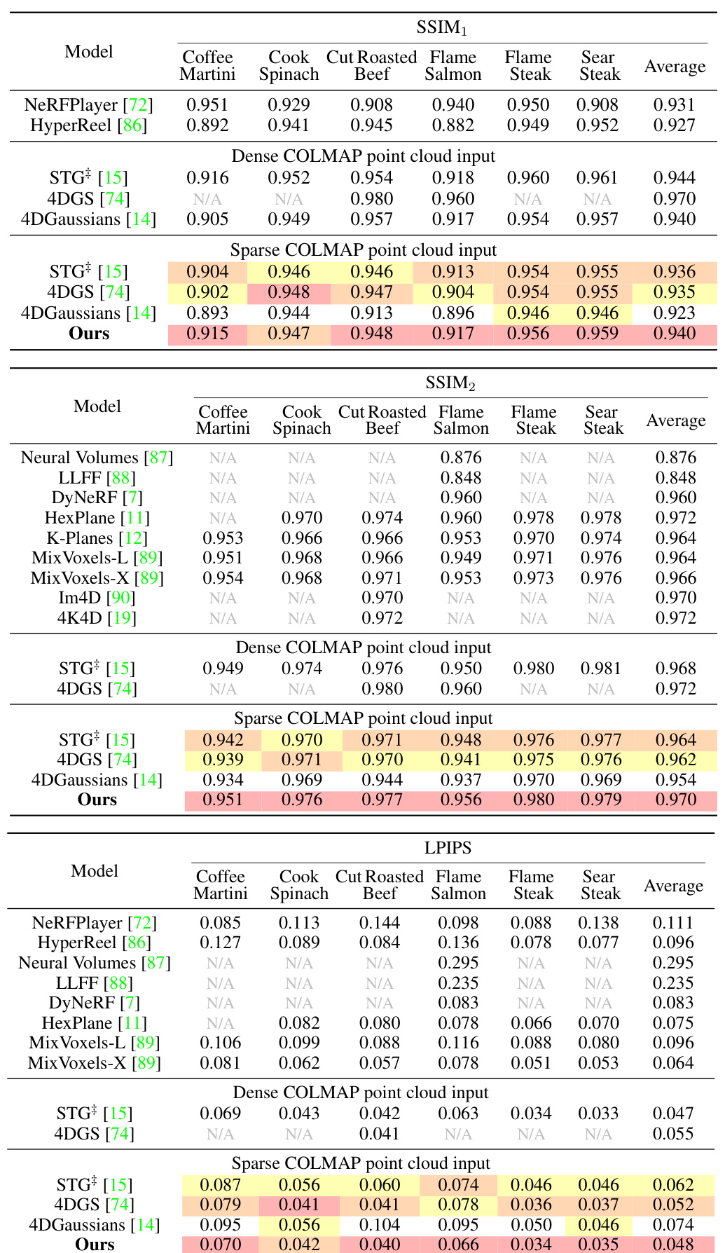
🔼 This table compares the proposed Ex4DGS method with other state-of-the-art dynamic Gaussian splatting methods on the Neural 3D Video dataset. It shows a comparison of PSNR, SSIM, and LPIPS scores, as well as training time (including preprocessing) and frames per second (FPS). The table also notes some differences in hardware and dataset sizes used for training among the various methods.
read the caption
Table 1: Comparison of ours with the comparison methods on Neural 3D Video dataset [7]. Training time: Both preprocessing and the accumulated time of all subsequent training phases. Both the training time and FPS are measured under the same machine with an NVIDIA 4090 GPU for strictly fair comparisons. †: STG is done with an H100 GPU machine due to the memory issue. ‡: Trained using a dataset split into 150 frames.
Full paper#

