TL;DR#
Current transfer learning methods struggle with limited data and domain shift. Task vectors, which represent the difference between pre-trained and task-specific model weights, offer potential solutions but suffer from interference when combined.
The paper proposes aTLAS, an algorithm that linearly combines parameter blocks of task vectors with learned coefficients, achieving anisotropic scaling. This method exploits the low intrinsic dimensionality of pre-trained models, enhancing knowledge composition and transfer. aTLAS shows significant improvements in task arithmetic, few-shot recognition, and test-time adaptation with limited or no labelled data.
Key Takeaways#
Why does it matter?#
This paper is important because it introduces a novel parameter-efficient fine-tuning method, aTLAS, that leverages the compositional properties of task vectors. This offers significant advantages in low-data regimes, few-shot learning, and test-time adaptation, addressing key challenges in current machine learning research. The modular approach and strong empirical results open exciting avenues for future research in knowledge transfer and efficient model adaptation. The focus on parameter efficiency makes it particularly relevant in the context of increasingly large foundation models.
Visual Insights#
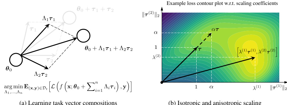
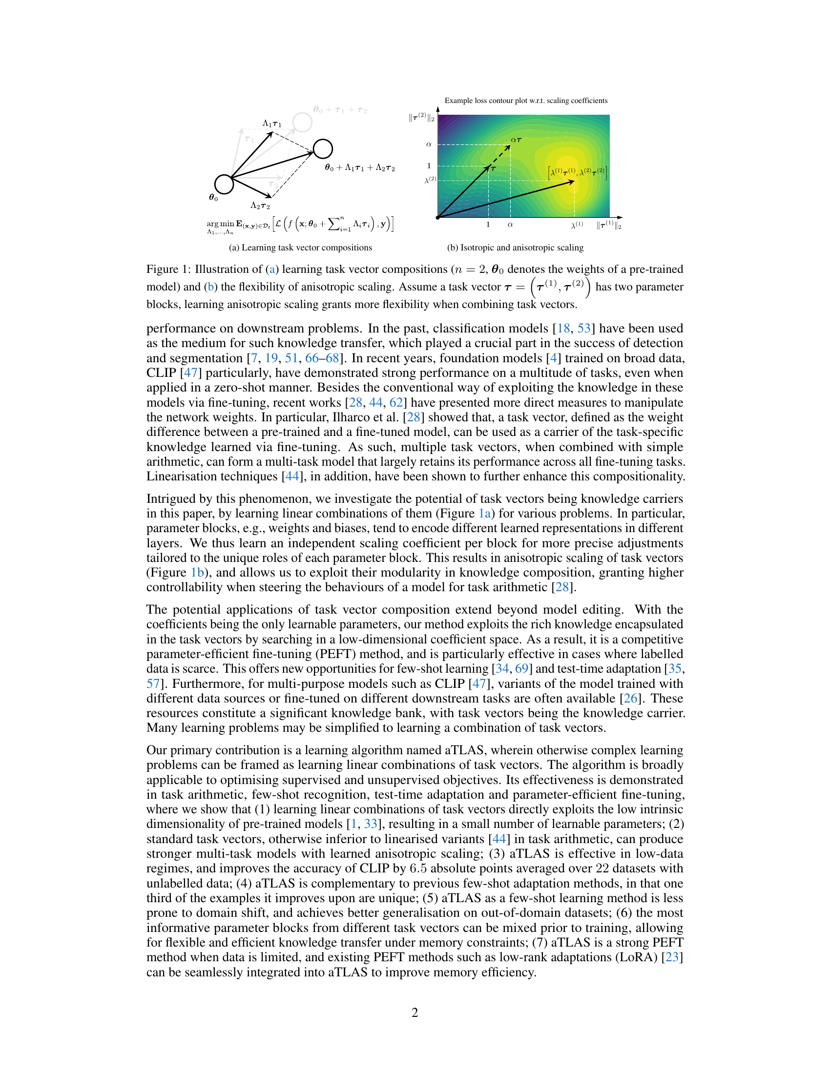
🔼 This figure illustrates the core idea of the aTLAS algorithm. Panel (a) shows how multiple task vectors (T1 and T2) are linearly combined with learned coefficients (λ1 and λ2) to form a composite task vector. This composite vector, when added to the pre-trained model weights (θ0), produces a new model adapted for a specific task. Panel (b) compares isotropic and anisotropic scaling. Isotropic scaling applies the same scaling factor to all parameter blocks within a task vector, while anisotropic scaling allows for different scaling factors for each block, offering greater flexibility in composing task vectors.
read the caption
Figure 1: Illustration of (a) learning task vector compositions (n = 2, θ0 denotes the weights of a pre-trained model) and (b) the flexibility of anisotropic scaling. Assume a task vector T = [T(1), T(2)] has two parameter blocks, learning anisotropic scaling grants more flexibility when combining task vectors.
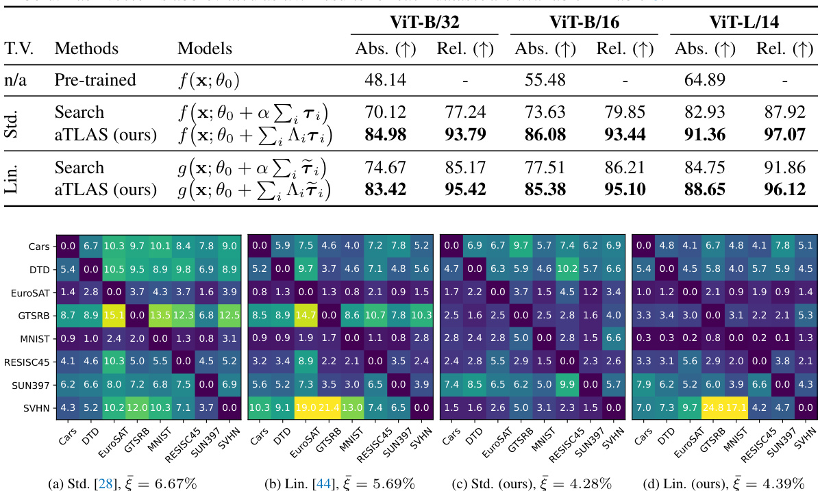
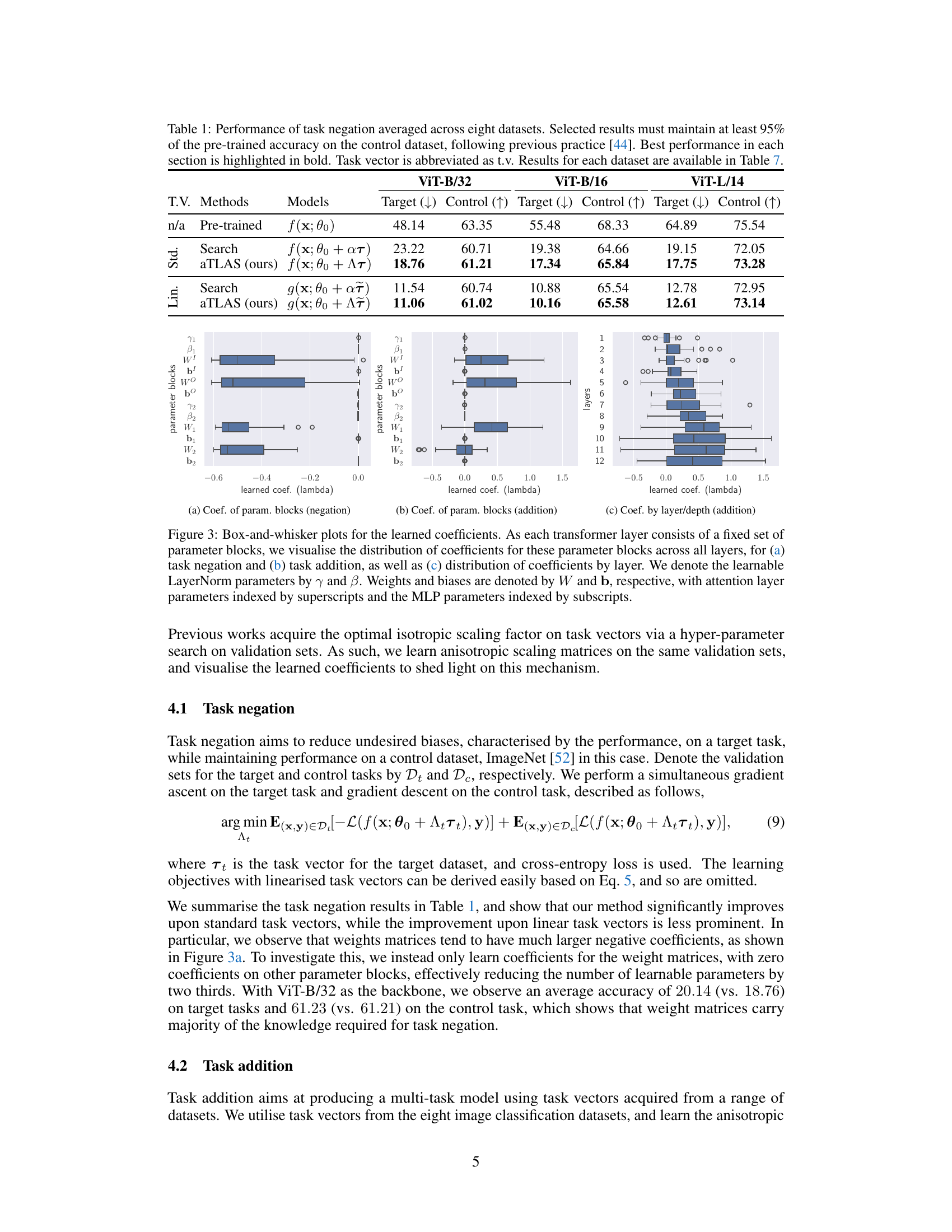
🔼 This table presents the results of task negation experiments conducted on eight image classification datasets. The task negation method aims to reduce undesired biases on a target task while maintaining performance on a control task (ImageNet). The table compares different methods, including a baseline (pre-trained model) and two variations of the proposed aTLAS method (using standard and linearized task vectors), with a standard search method. The results show the target and control task accuracies for each method, with the best-performing method highlighted in bold for each dataset and model size.
read the caption
Table 1: Performance of task negation averaged across eight datasets. Selected results must maintain at least 95% of the pre-trained accuracy on the control dataset, following previous practice [44]. Best performance in each section is highlighted in bold. Task vector is abbreviated as t.v. Results for each dataset are available in Table 7.
In-depth insights#
Anisotropic Scaling#
Anisotropic scaling, in the context of this research paper, is a crucial technique for enhancing knowledge composition and transfer in pre-trained models. Unlike isotropic scaling, which uniformly scales all parameters, anisotropic scaling allows for independent scaling of different parameter blocks, such as weights and biases in different layers of a neural network. This approach leverages the understanding that different parts of a model capture different levels of knowledge representation. By learning separate scaling coefficients for each parameter block, the algorithm efficiently exploits the low intrinsic dimensionality of the model while achieving greater flexibility in task vector composition. This results in more disentangled task vectors, reducing interference during composition and leading to improved performance in task arithmetic and other downstream applications. Furthermore, this granular control over the scaling process leads to a more parameter-efficient fine-tuning method, particularly beneficial when dealing with limited labelled data or when aiming for better generalizability in low-data regimes. The effectiveness of anisotropic scaling is demonstrated empirically across various tasks, including few-shot learning and test-time adaptation.
Task Vector Composition#
The concept of “Task Vector Composition” centers on the idea of combining learned representations from different tasks to create a more powerful and versatile model. Task vectors, which represent the difference in model parameters between a pre-trained model and a task-specific fine-tuned model, become fundamental building blocks. The core idea is that these vectors encapsulate the knowledge gained during fine-tuning and, under the right conditions (such as linear combinations or simple arithmetic operations), can be added to the pre-trained model to adapt it to new or combined tasks. This modular approach allows for a more efficient and flexible form of transfer learning, especially in low-data regimes, as existing knowledge is leveraged. However, challenges exist in disentangling the task vectors to prevent interference when combining them, and understanding the relative informativeness of different parameter blocks within those vectors is crucial for effective composition. The optimal combination strategy involves learning scaling coefficients or matrices to balance the contributions of individual task vectors during adaptation, moving beyond simple arithmetic addition. The method’s efficacy hinges on the inherent low intrinsic dimensionality of pre-trained models which allow for successful transfer and modular learning.
Low-Data Regime#
The concept of a ‘Low-Data Regime’ in machine learning is crucial because it addresses the challenge of training effective models with limited labeled data. This is especially relevant for many real-world scenarios where acquiring large annotated datasets can be expensive, time-consuming, or even impossible. The core idea is to leverage transfer learning or other techniques that can effectively utilize prior knowledge or limited data to achieve reasonably good performance. In this context, the paper likely explores methods that enhance the capabilities of models trained on limited data, potentially including techniques such as parameter-efficient fine-tuning, data augmentation, and learning strategies that promote generalization from few examples. The ‘Low-Data Regime’ section would likely showcase the performance of these methods on benchmark datasets, demonstrating their effectiveness compared to conventional approaches that assume abundance of data. Success in this area would highlight the practicality and scalability of the proposed approach in situations with limited resources.
PEFT & Scalability#
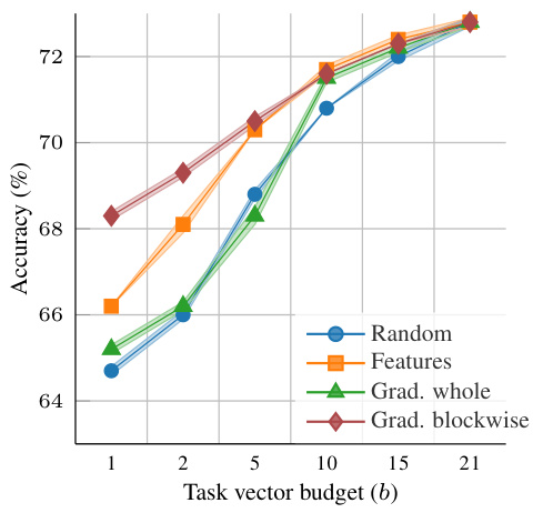
Parameter-efficient fine-tuning (PEFT) methods are crucial for adapting large language models to specific tasks without excessive computational cost. The paper explores this by framing the problem as learning linear combinations of task vectors, enabling efficient knowledge transfer. Anisotropic scaling, applied at the task vector level, provides flexibility by independently scaling different parameter blocks, allowing for more precise adjustments than isotropic scaling. This modular approach leverages already-learned representations, reducing dependence on large datasets and showing efficacy in few-shot and test-time adaptation. aTLAS, the proposed algorithm, demonstrates significant parameter efficiency through its use of only linear combination coefficients as learnable parameters. However, the paper acknowledges scalability as a potential limitation when sufficient training data is available. A strategy to address this involves partitioning parameter blocks and learning individual coefficients for each partition, effectively scaling up learnable parameters. This allows aTLAS to achieve higher accuracy with more training data, while maintaining its parameter efficiency. The integration of PEFT methods such as LoRA further enhances aTLAS’s efficiency and scalability. Overall, the approach strikes a balance between accuracy and efficiency, making it a promising PEFT technique.
Limitations & Future#
The research paper’s ‘Limitations & Future’ section would critically examine the constraints of the proposed aTLAS method. This might include its reliance on pre-trained models, potentially limiting its applicability to tasks where suitable pre-trained models are unavailable. The discussion should address the scalability challenges, especially when handling a large number of task vectors or adapting it for models with a vastly increased parameter count. The impact of the limited number of learnable parameters on model performance, particularly with abundant training data, should be acknowledged. A key area for future work would explore more sophisticated task vector selection strategies to improve efficiency and performance. Furthermore, investigations into the integration of aTLAS with other PEFT methods, exploring potential synergies or overcoming limitations, would offer interesting avenues for future exploration. Finally, exploring aTLAS’s application on a wider variety of tasks and datasets will expand the study and offer more insights into the generalization capabilities of the method and the compositional properties of task vectors.
More visual insights#
More on figures

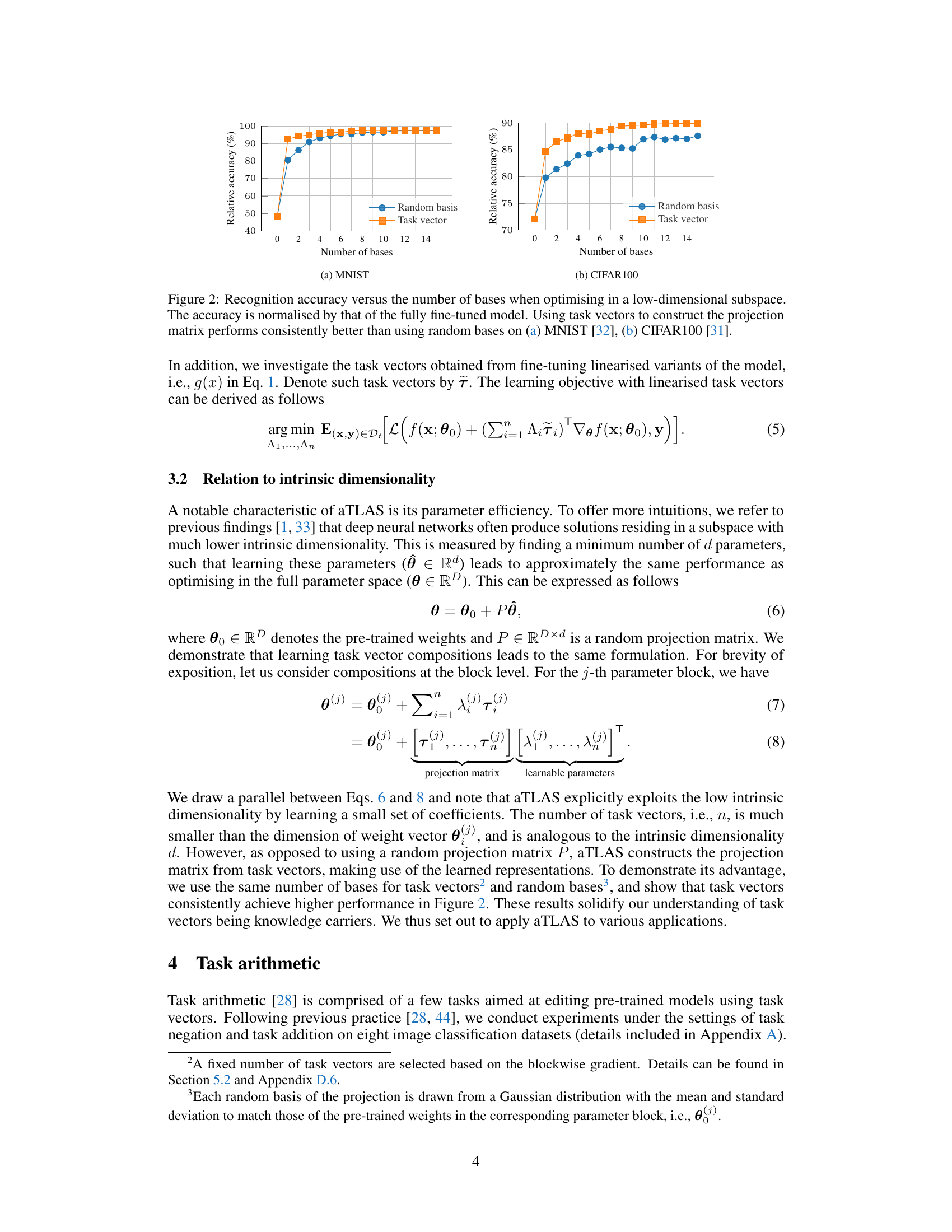
🔼 This figure compares the performance of using task vectors versus random bases for dimensionality reduction in few-shot image classification. The results show that using task vectors to construct the projection matrix consistently leads to higher accuracy compared to random bases, particularly on MNIST and CIFAR100 datasets. The accuracy is normalized relative to a fully fine-tuned model, highlighting the efficiency of the task vector approach.
read the caption
Figure 2: Recognition accuracy versus the number of bases when optimising in a low-dimensional subspace. The accuracy is normalised by that of the fully fine-tuned model. Using task vectors to construct the projection matrix performs consistently better than using random bases on (a) MNIST [32], (b) CIFAR100 [31].
🔼 This figure illustrates two key concepts of the aTLAS algorithm. (a) shows how task vector compositions are learned by linearly combining multiple task vectors (T1, T2, etc.) with learned coefficients (λ1, λ2, etc.). The pre-trained model’s weights are represented by θ0. (b) highlights the advantage of anisotropic scaling over isotropic scaling. Anisotropic scaling allows for independent scaling of different parameter blocks within a task vector, providing greater flexibility in combining task vectors. This is visualized with an example of a loss contour plot, demonstrating how anisotropic scaling allows for more efficient optimization.
read the caption
Figure 1: Illustration of (a) learning task vector compositions (n = 2, 00 denotes the weights of a pre-trained model) and (b) the flexibility of anisotropic scaling. Assume a task vector T = T(1), T(2) has two parameter blocks, learning anisotropic scaling grants more flexibility when combining task vectors.

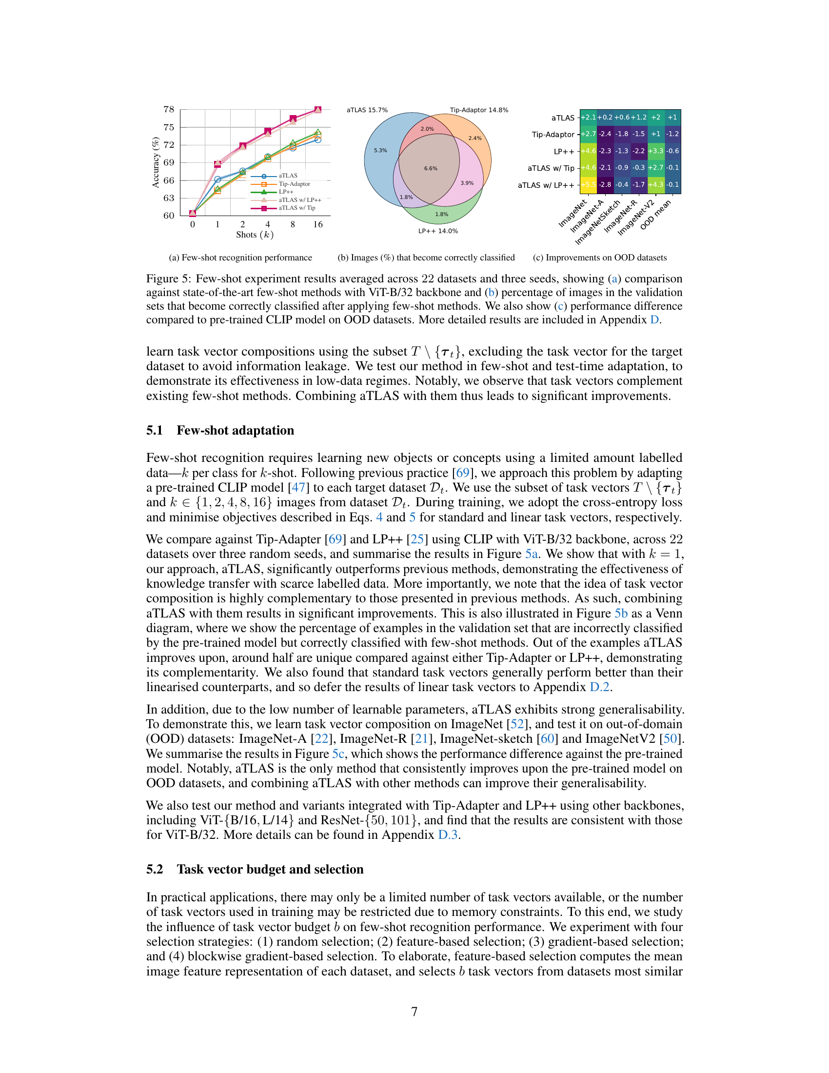
🔼 This figure presents the results of few-shot learning experiments conducted on 22 datasets using three different methods: aTLAS, Tip-Adapter, and LP++. Subfigure (a) compares the accuracy of these methods across different numbers of training examples (shots), demonstrating aTLAS’s superior performance. Subfigure (b) illustrates, through a Venn diagram, the number of images correctly classified by each method that were misclassified by the pretrained CLIP model, highlighting aTLAS’s unique contributions. Finally, subfigure (c) shows the improvement in accuracy achieved by each method on out-of-distribution (OOD) datasets, revealing aTLAS’s robustness and generalizability.
read the caption
Figure 5: Few-shot experiment results averaged across 22 datasets and three seeds, showing (a) comparison against state-of-the-art few-shot methods with ViT-B/32 backbone and (b) percentage of images in the validation sets that become correctly classified after applying few-shot methods. We also show (c) performance difference compared to pre-trained CLIP model on OOD datasets. More detailed results are included in Appendix D.
🔼 This figure shows the results of an experiment comparing the performance of using task vectors versus random bases for constructing a projection matrix in a low-dimensional subspace. The accuracy is normalized to that of a fully fine-tuned model. The results, shown for MNIST and CIFAR100 datasets, demonstrate that using task vectors consistently outperforms using random bases.
read the caption
Figure 2: Recognition accuracy versus the number of bases when optimising in a low-dimensional subspace. The accuracy is normalised by that of the fully fine-tuned model. Using task vectors to construct the projection matrix performs consistently better than using random bases on (a) MNIST [32], (b) CIFAR100 [31].

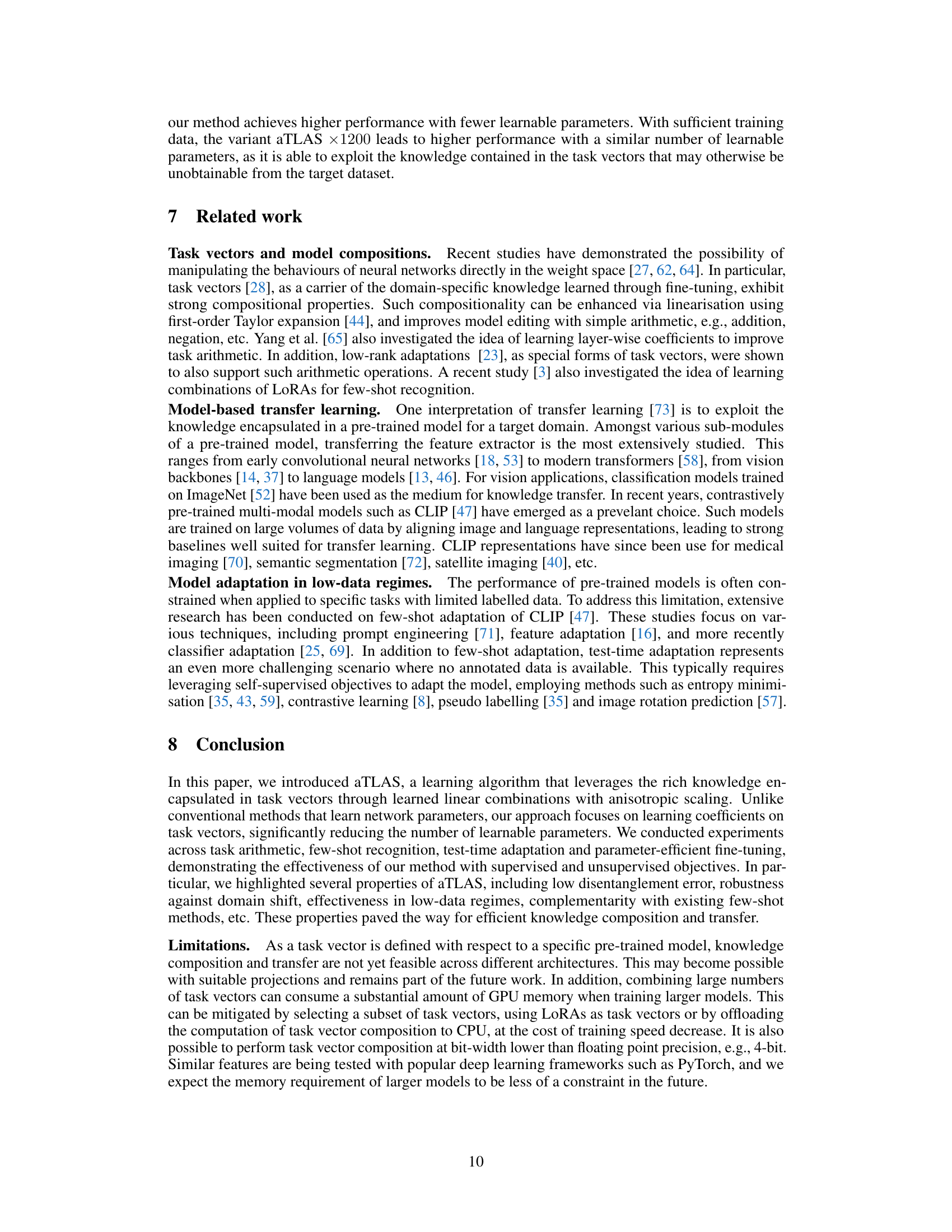
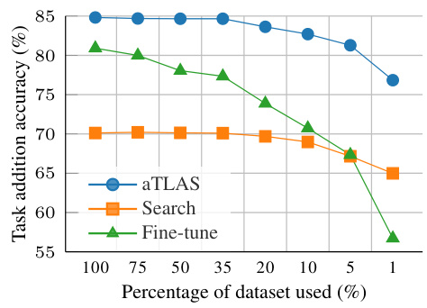
🔼 This figure shows how the performance of aTLAS scales with the amount of training data. It compares aTLAS with different numbers of learnable parameters (2k, 10k, 40k, 160k, and 2.4M) against LoRA (2.4M). The x-axis represents the percentage of training data used, and the y-axis shows the average accuracy across 22 datasets. The results demonstrate that aTLAS’s performance improves as the number of learnable parameters and the amount of training data increase, and that it becomes competitive with LoRA when sufficient data is available.
read the caption
Figure 7: Scalability of aTLAS. We compare the accuracy of our method against LoRAs, and vary the amount of training data. Results are averaged over 22 datasets. Detailed results are included in Table 17.

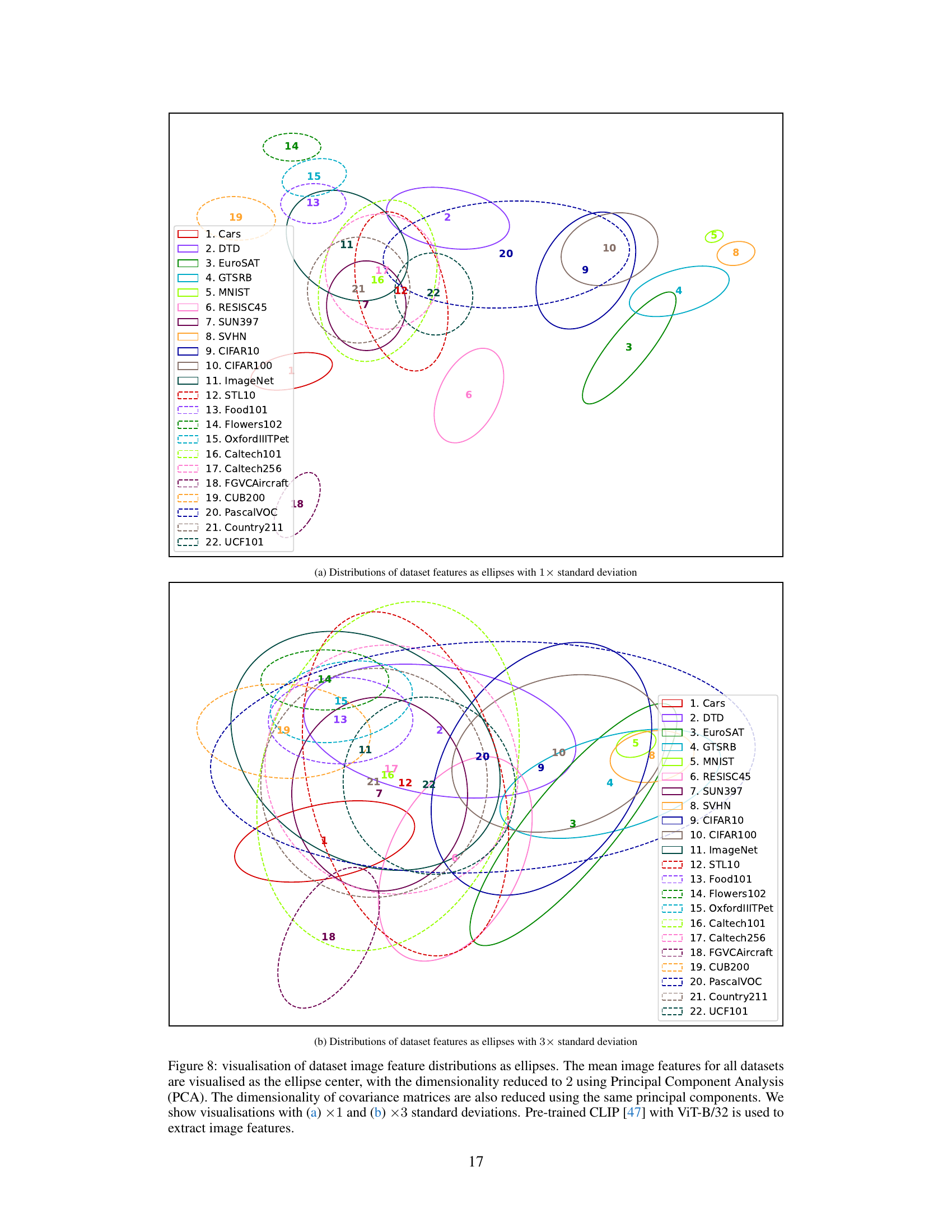
🔼 This figure visualizes the distributions of image features extracted from 22 different datasets using Principal Component Analysis (PCA) to reduce dimensionality to 2. The mean features of each dataset are represented by the center of an ellipse, and the covariance matrix is used to determine the shape and size of the ellipse. The visualizations are shown with both 1 and 3 standard deviations, providing a visual representation of the spread of the image features for each dataset. This helps to illustrate the relationships and similarities between different image datasets.
read the caption
Figure 8: visualisation of dataset image feature distributions as ellipses. The mean image features for all datasets are visualised as the ellipse center, with the dimensionality reduced to 2 using Principal Component Analysis (PCA). The dimensionality of covariance matrices are also reduced using the same principal components. We show visualisations with (a) ×1 and (b) ×3 standard deviations. Pre-trained CLIP [47] with ViT-B/32 is used to extract image features.
🔼 This figure illustrates two key concepts of the aTLAS algorithm. (a) shows how task vectors, which represent the difference in weights between a pre-trained model and a model fine-tuned for a specific task, can be linearly combined to create new representations. The coefficients of the linear combination are learned parameters. (b) highlights that anisotropic scaling, where different parameter blocks within a task vector are scaled differently, provides greater flexibility in composing task vectors compared to isotropic scaling (where all blocks are scaled equally). Anisotropic scaling allows for a more nuanced and efficient combination of task-specific knowledge.
read the caption
Figure 1: Illustration of (a) learning task vector compositions (n = 2, 00 denotes the weights of a pre-trained model) and (b) the flexibility of anisotropic scaling. Assume a task vector T = T(1) (2) has two parameter blocks, learning anisotropic scaling grants more flexibility when combining task vectors.
🔼 This figure shows two illustrations. The first one (a) illustrates how to learn task vector compositions using a pre-trained model and two task vectors. The second one (b) illustrates the flexibility of anisotropic scaling, assuming a task vector with two parameter blocks. In summary, this figure explains the main idea of the proposed method, aTLAS.
read the caption
Figure 1: Illustration of (a) learning task vector compositions (n = 2, θ0 denotes the weights of a pre-trained model) and (b) the flexibility of anisotropic scaling. Assume a task vector τ = (τ(1), τ(2)) has two parameter blocks, learning anisotropic scaling grants more flexibility when combining task vectors.
🔼 This figure illustrates the core idea of the aTLAS algorithm proposed in the paper. Panel (a) shows how task vector compositions are learned by linearly combining multiple task vectors (T1 and T2 in this case) with learned coefficients (α1 and α2). The pre-trained model weights (θ0) are also included in the composition. Panel (b) demonstrates the difference between isotropic and anisotropic scaling. Anisotropic scaling allows for independent scaling of different components (blocks) of the task vector, providing more flexibility in combining task vectors and thus enhancing the knowledge composition process. The example loss contour plot shows how anisotropic scaling allows finding a more flexible and accurate optimal point compared to isotropic scaling, illustrating the advantage of the method.
read the caption
Figure 1: Illustration of (a) learning task vector compositions (n = 2, θ0 denotes the weights of a pre-trained model) and (b) the flexibility of anisotropic scaling. Assume a task vector T = T(1),T(2) has two parameter blocks, learning anisotropic scaling grants more flexibility when combining task vectors.
🔼 This figure illustrates two key concepts of the paper: task vector composition and anisotropic scaling. Panel (a) shows how multiple task vectors (representing knowledge learned for different tasks) can be combined linearly to create a new representation. The weights of a pre-trained model (θ₀) serve as a baseline, and learned scaling coefficients (λ₁, λ₂) adjust the contribution of each task vector. Panel (b) highlights the advantage of anisotropic scaling. Isotropic scaling would uniformly scale all parameter blocks within a task vector, limiting flexibility. Anisotropic scaling, however, scales each parameter block (e.g., weights, biases) independently with a unique coefficient, leading to greater flexibility in composing task vectors.
read the caption
Figure 1: Illustration of (a) learning task vector compositions (n = 2, 00 denotes the weights of a pre-trained model) and (b) the flexibility of anisotropic scaling. Assume a task vector T = has two parameter blocks, learning anisotropic scaling grants more flexibility when combining task vectors.

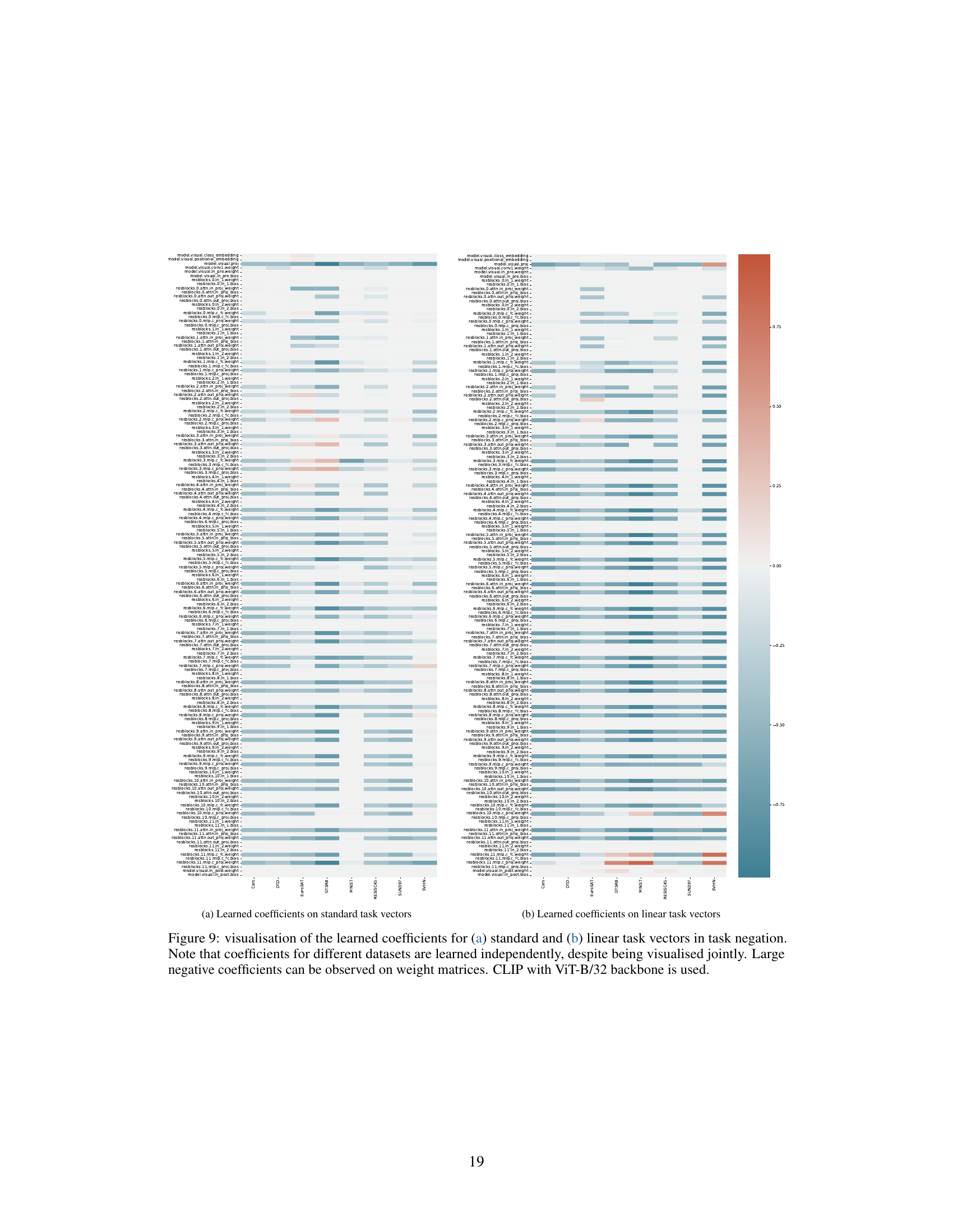
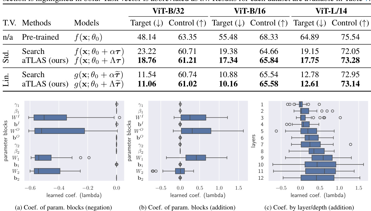
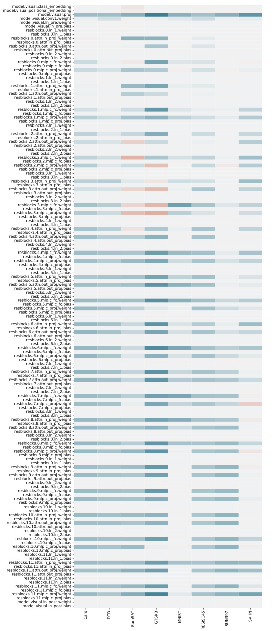
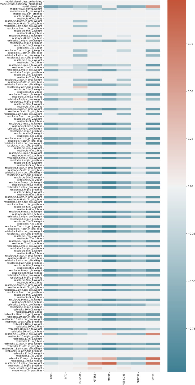
🔼 This figure visualizes the learned coefficients for both standard and linearized task vectors during task negation. Each row represents a different parameter block within the model, and each column corresponds to one of the eight datasets used in the experiment. The heatmap shows the learned coefficients, with warmer colors indicating larger (more positive) values and cooler colors indicating smaller (more negative) values. The visualization highlights that weight matrices tend to learn large negative coefficients in the task negation process, and the coefficients for different datasets are learned independently.
read the caption
Figure 9: visualisation of the learned coefficients for (a) standard and (b) linear task vectors in task negation. Note that coefficients for different datasets are learned independently, despite being visualised jointly. Large negative coefficients can be observed on weight matrices. CLIP with ViT-B/32 backbone is used.

🔼 This figure illustrates the core idea of the paper, which is to improve task vector composition by learning anisotropic scaling. Panel (a) shows how task vectors (T1, T2) from different domains are linearly combined with learned coefficients (A1, A2). Panel (b) visually demonstrates the concept of anisotropic scaling where the different components or blocks of the task vectors (represented as a vector) are weighted differently compared to isotropic scaling where each component would be equally weighted. This anisotropic scaling enables more flexible composition as different components can be weighted differently according to their relevance to the target task.
read the caption
Figure 1: Illustration of (a) learning task vector compositions (n = 2, 00 denotes the weights of a pre-trained model) and (b) the flexibility of anisotropic scaling. Assume a task vector T = has two parameter blocks, learning anisotropic scaling grants more flexibility when combining task vectors.
More on tables

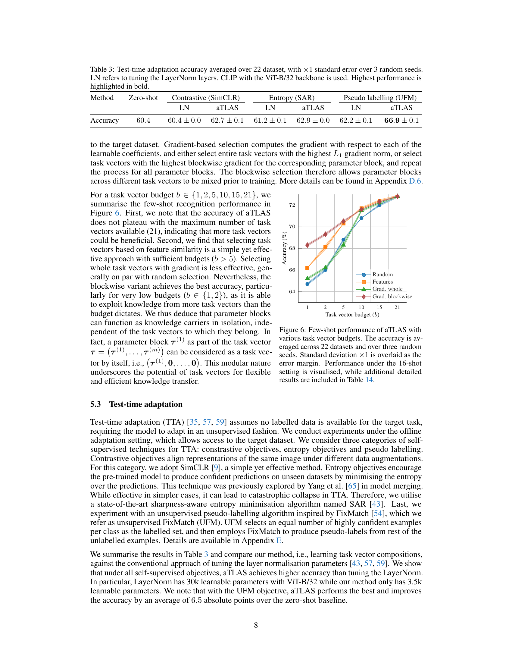
🔼 This table shows the results of test-time adaptation experiments using different methods. Test-time adaptation is a technique where the model adapts to a new task without using labeled data. The results are averaged across 22 different datasets. The table compares several methods, including tuning the LayerNorm layers (LN) and using aTLAS, and shows the accuracy achieved with each method along with standard error calculated over 3 independent runs.
read the caption
Table 3: Test-time adaptation accuracy averaged over 22 dataset, with ×1 standard error over 3 random seeds. LN refers to tuning the LayerNorm layers. CLIP with the ViT-B/32 backbone is used. Highest performance is highlighted in bold.

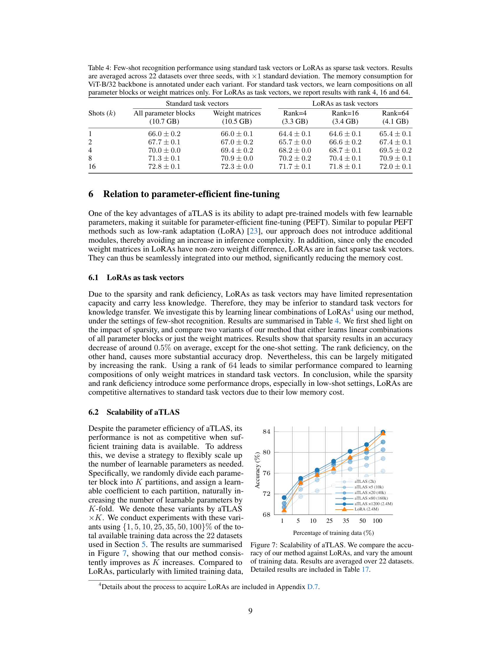
🔼 This table presents the few-shot recognition performance results using different task vector types and methods. The results are averaged across 22 datasets and three random seeds, with standard deviations reported. The table compares the performance of using standard task vectors (all parameter blocks and weight matrices only) with LoRAs (low-rank adaptation) as sparse task vectors, for ranks 4, 16, and 64. Memory consumption for the ViT-B/32 backbone is also shown.
read the caption
Table 4: Few-shot recognition performance using standard task vectors or LoRAs as sparse task vectors. Results are averaged across 22 datasets over three seeds, with ×1 standard deviation. The memory consumption for ViT-B/32 backbone is annotated under each variant. For standard task vectors, we learn compositions on all parameter blocks or weight matrices only. For LoRAs as task vectors, we report results with rank 4, 16 and 64.

🔼 This table provides a comprehensive overview of the 22 image classification datasets used in the paper’s experiments. For each dataset, it lists the number of classes, the sizes of the training, validation, and testing splits, the number of training epochs, and the fine-tuned accuracy achieved using various backbones of the CLIP model (RN50, RN101, ViT-B/32, ViT-B/16, and ViT-L/14). This information is crucial for understanding the experimental setup and evaluating the performance of the proposed method across diverse datasets.
read the caption
Table 5: Details of the 22 image classification datasets used in experiments, the number of epochs for fine-tuning and the final accuracy for different backbones of the CLIP model.

🔼 This table shows the learning rates and number of training epochs used for the task negation experiments on eight different datasets. The learning rate and number of epochs were determined using a hyperparameter search on the validation set for each dataset. This table is essential for reproducing the results of the task negation experiments.
read the caption
Table 6: Learning rates and training epochs for task negation.

🔼 This table presents the performance of task negation on eight image classification datasets using different methods. The results show the accuracy on both the target and control tasks. The control task ensures that the method maintains a certain level of performance on a general dataset. The best performing method in each dataset and overall is highlighted in bold. Abbreviations: t.v. = task vector.
read the caption
Table 1: Performance of task negation averaged across eight datasets. Selected results must maintain at least 95% of the pre-trained accuracy on the control dataset, following previous practice [44]. Best performance in each section is highlighted in bold. Task vector is abbreviated as t.v. Results for each dataset are available in Table 7.

🔼 This table presents the performance comparison of different methods on task negation across eight image classification datasets. The results are evaluated based on accuracy on both target and control tasks. The table compares standard task vector methods (with and without learned anisotropic scaling) and linearized task vector methods (also with and without learned anisotropic scaling). The best-performing method for each setting is highlighted in bold, and complete results for each dataset are available in another table referenced in the caption.
read the caption
Table 1: Performance of task negation averaged across eight datasets. Selected results must maintain at least 95% of the pre-trained accuracy on the control dataset, following previous practice [44]. Best performance in each section is highlighted in bold. Task vector is abbreviated as t.v. Results for each dataset are available in Table 7.

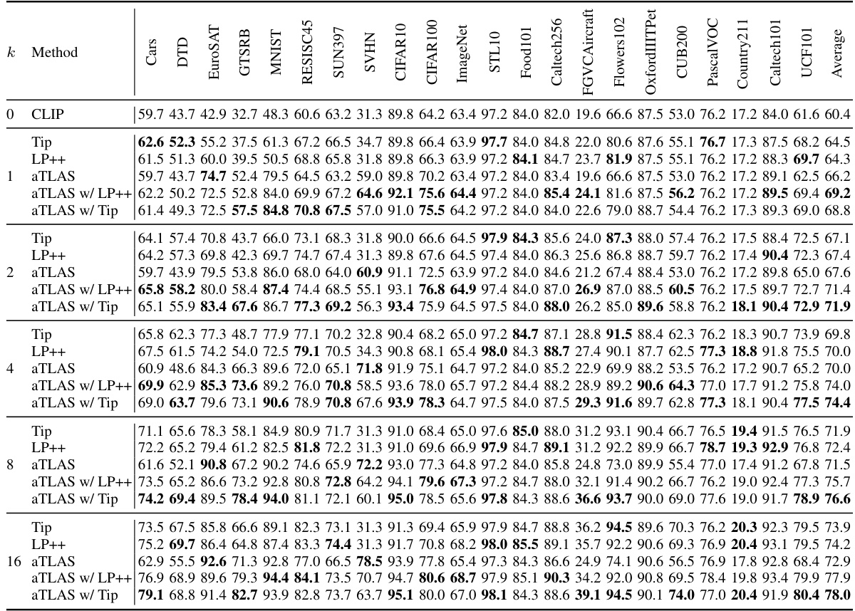
🔼 This table presents the average accuracy of different few-shot learning methods across 22 image recognition datasets. The results are obtained using the CLIP model with a ViT-B/32 backbone. The table shows the performance for different numbers of shots (k) including 1, 2, 4, 8, and 16. It compares the performance of the Tip-Adapter, LP++, and aTLAS methods (with both standard and linearised task vectors). The best-performing method for each shot is highlighted in bold.
read the caption
Table 9: Average accuracy for few-shot recognition over 22 datasets. We report accuracy averaged over 3 random n-shot sample selections, with 1× standard error. Results are produced using CLIP with ViT-B/32 backbone. For our method, we show results with both standard [28] and linearised [44] task vectors. The best method for each choice of k ∈ {1, 2, 4, 8, 16} is highlighted in bold.

🔼 This table presents the results of task negation experiments conducted on eight image classification datasets. The task negation aims to reduce undesired biases on a target task while maintaining performance on a control dataset (ImageNet). The table compares different methods, including standard task vectors (t.v.), linearised task vectors, and the proposed aTLAS method. Results include target and control dataset performance metrics and highlights the best-performing method for each. More detailed results for each dataset are provided in a separate table (Table 7).
read the caption
Table 1: Performance of task negation averaged across eight datasets. Selected results must maintain at least 95% of the pre-trained accuracy on the control dataset, following previous practice [44]. Best performance in each section is highlighted in bold. Task vector is abbreviated as t.v. Results for each dataset are available in Table 7.
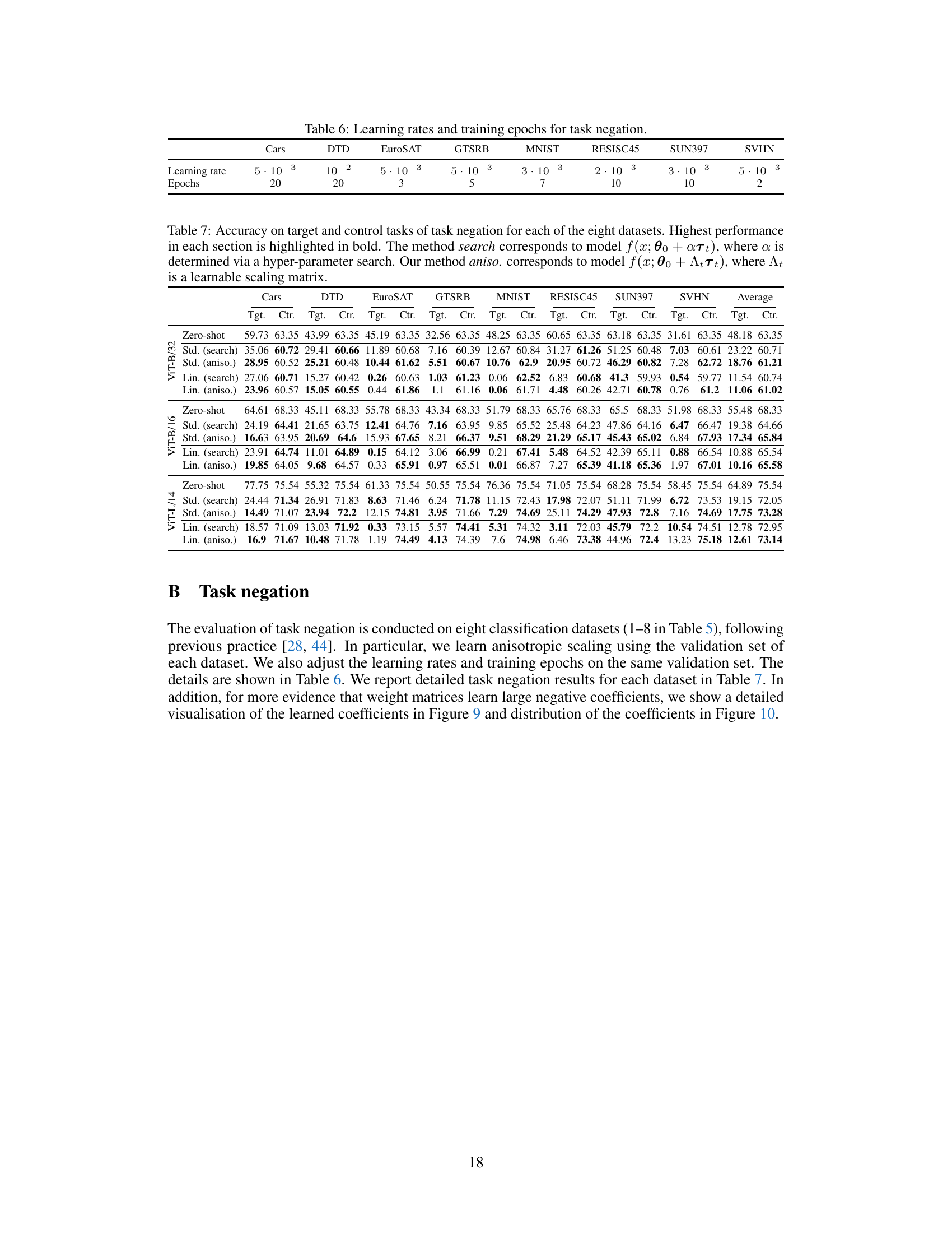
🔼 This table presents the results of task negation experiments on eight image classification datasets. It compares the performance of several methods, including zero-shot, standard task vector search (isotropic), anisotropic task vector scaling (our proposed method), linear task vector search, and linear anisotropic task vector scaling. For each method, target and control task accuracies are shown for three ViT models (ViT-L/14, ViT-B/32, ViT-B/16). The table highlights the best performing method for each dataset and model size.
read the caption
Table 7: Accuracy on target and control tasks of task negation for each of the eight datasets. Highest performance in each section is highlighted in bold. The method search corresponds to model f(x; θ0 + αTτ), where α is determined via a hyper-parameter search. Our method aniso. corresponds to model f(x; θ0 + Aττ), where Aτ is a learnable scaling matrix.

🔼 This table presents the results of task negation experiments on eight image classification datasets. It compares the performance of different methods, including a baseline (zero-shot), a hyperparameter search method, and the proposed aTLAS method (with both standard and linearised task vectors) on both target and control tasks. The results are given for three different ViT model sizes. The table highlights the effectiveness of the aTLAS method in achieving strong performance on the target task while maintaining performance on the control task, especially in comparison to the hyperparameter search method.
read the caption
Table 7: Accuracy on target and control tasks of task negation for each of the eight datasets. Highest performance in each section is highlighted in bold. The method search corresponds to model f(x; θ0 + αT ), where α is determined via a hyper-parameter search. Our method aniso. corresponds to model f(x; θ0 + AT ), where AT is a learnable scaling matrix.

🔼 This table presents the results of task negation experiments conducted on eight image classification datasets. The task negation technique aims to reduce undesired biases on a target task while maintaining performance on a control task (ImageNet). The table compares the performance of several methods: a pre-trained model, a linear standard search method using task vectors, aTLAS (the proposed method), and similar approaches using linearised task vectors. The results are shown in terms of accuracy on both the target and control tasks, highlighting the best-performing method for each dataset. More detailed results for each dataset are provided in a separate table (Table 7).
read the caption
Table 1: Performance of task negation averaged across eight datasets. Selected results must maintain at least 95% of the pre-trained accuracy on the control dataset, following previous practice [44]. Best performance in each section is highlighted in bold. Task vector is abbreviated as t.v. Results for each dataset are available in Table 7.

🔼 This table presents the average accuracy for few-shot recognition across 22 different datasets. The results are obtained using the CLIP model with the ViT-B/32 backbone. Three different random n-shot sample selections are used, and the standard error is reported alongside the accuracy. The table compares the performance of the proposed aTLAS method to existing Tip-Adapter and LP++ methods, across various numbers of shots (k=1,2,4,8,16). Both standard and linearized versions of the aTLAS task vectors are included for comparison.
read the caption
Table 9: Average accuracy for few-shot recognition over 22 datasets. We report accuracy averaged over 3 random n-shot sample selections, with 1× standard error. Results are produced using CLIP with ViT-B/32 backbone. For our method, we show results with both standard [28] and linearised [44] task vectors. The best method for each choice of k ∈ {1, 2, 4, 8, 16} is highlighted in bold.

🔼 This table presents the few-shot learning performance of aTLAS using different LoRA configurations. It compares the results of aTLAS using LoRAs trained only on attention layers, only on MLP layers, and on both attention and MLP layers. For each LoRA configuration, it shows the performance of aTLAS alone, and also when combined with LP++ and Tip-Adapter, two other state-of-the-art few-shot learning methods. The results are averaged over 22 datasets and three random seeds. The table is designed to show the impact of different LoRA training strategies on the overall performance, and how combining aTLAS with other techniques affects the final accuracy.
read the caption
Table 15: Additional few-shot recognition results using LoRAs trained on attention layers, MLP layers or both. Results are averaged across 22 datasets over three seeds, with ×1 standard deviation. Rank 16 is used for LoRAs.

🔼 This table presents the few-shot recognition performance results using gradient-free optimization. The results are averaged across 22 different datasets and include standard error values, calculated from three separate random seeds. The table shows the performance for different numbers of shots (1, 2, 4, 8, 16) under different scaling methods (anisotropic with gradient and isotropic without gradient). The memory consumption in GB is also specified for each method.
read the caption
Table 16: Few-shot recognition performance with gradient-free optimization. Results are averaged accuracy over 22 datasets, with ×1 standard error over 3 random seeds.

🔼 This table shows the accuracy of different aTLAS variants and LoRA, when fine-tuned using different percentages of training data. The aTLAS variants systematically increase the number of learnable parameters. The results demonstrate how the accuracy improves with more data and more parameters, although the improvements diminish with larger models.
read the caption
Table 17: Accuracy after fine-tuning on different percentage of training data for variants of aTLAS × K and LoRAs [23]. Results are averaged across 22 datasets. Highest accuracy in each section is highlighted in bold.
Full paper#

