TL;DR#
Estimating the joint probability density of high-dimensional data is a crucial challenge in machine learning and statistics. Existing methods, like those based on Markov Chain Monte Carlo (MCMC) or normalizing flows, often struggle with computational cost and data requirements, particularly when dealing with high dimensionality. Additionally, many existing methods make restrictive assumptions on data structure which limits their applicability.
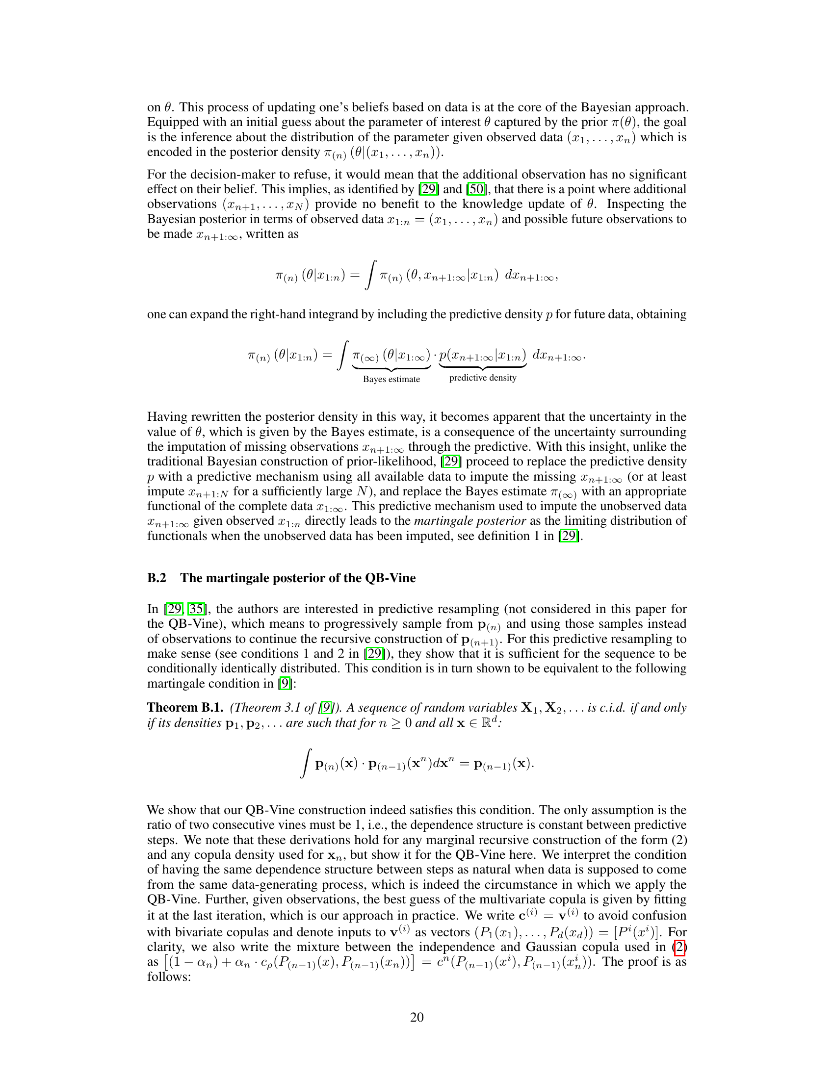
The paper introduces a new method called Quasi-Bayesian Vine (QB-Vine). This innovative approach cleverly decomposes the high-dimensional density into one-dimensional marginal densities and a copula, which models the dependencies between the dimensions. Using highly expressive vine copulas combined with efficient Quasi-Bayesian recursive construction for marginal densities, it creates a fully non-parametric density estimator that is flexible, data-efficient and computationally faster than existing methods. Experiments on several high dimensional datasets show it significantly outperforms existing analytical methods.
Key Takeaways#
Why does it matter?#
This paper is significant as it presents a novel, data-efficient approach for high-dimensional density estimation. It leverages copula theory and Quasi-Bayesian methods, offering a computationally advantageous alternative to existing methods. This opens avenues for research in high-dimensional Bayesian inference and related machine learning tasks, particularly where large datasets are unavailable.
Visual Insights#

🔼 The figure shows the performance comparison of different density estimation methods on the Digits dataset, with a focus on the QB-Vine’s performance with varying training set sizes. The x-axis represents the training sample size, while the y-axis represents the average log predictive score (LPS) in bits per dimension (bpd). The plot illustrates the QB-Vine’s data efficiency, showing competitive performance with only 50 training samples and outperforming other methods significantly once the training size exceeds 200.
read the caption
Figure 1: Density estimation on the Digits data (n = 1797, d = 64) with reduced training sizes for the QB-Vine against other models fitted on the full training set. The QB-Vine achieves competitive performance for training sizes as little as n = 50 and outperforms all competitors once n > 200.
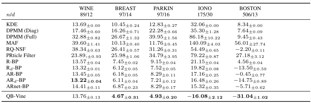
🔼 This table presents the average log predictive scores for density estimation on five different datasets using various methods, including the proposed QB-Vine method and several state-of-the-art baselines. The table highlights the QB-Vine’s superior performance, particularly as dimensionality increases. Error bars represent two standard deviations from the mean over five runs, indicating the variability of each method’s performance.
read the caption
Table 1: Average log predictive score (lower is better) with error bars corresponding to two standard deviations over five runs for density estimation on datasets analysed by [35]. We note that as dimension increases, the QB-Vine outperforms all benchmarks.
In-depth insights#
QB-Vine: A New Model#
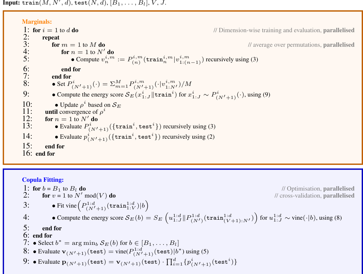
The proposed QB-Vine model presents a novel approach to high-dimensional density estimation by cleverly combining quasi-Bayesian methods with vine copulas. The core innovation lies in its ability to handle high-dimensional data without the restrictive assumptions often imposed by existing multivariate quasi-Bayesian methods. This is achieved through a copula decomposition, separating the joint predictive distribution into manageable one-dimensional marginals (handled efficiently by the R-BP algorithm) and a high-dimensional copula (modeled flexibly using vine copulas). This decomposition allows for parallel computation, significantly improving efficiency, especially for larger dimensions. The method’s theoretical foundation is supported by proving convergence rates that are, under certain conditions, independent of dimensionality. Empirical results demonstrate that QB-Vine significantly outperforms state-of-the-art methods on various benchmark datasets for density estimation and supervised learning tasks. However, the reliance on simplified vine copulas, while computationally advantageous, might represent a limitation in scenarios with complex, high-order dependencies. Future work could investigate more expressive copula models to enhance the model’s flexibility and accuracy.
Copula Decomposition#
Copula decomposition is a crucial technique for high-dimensional density estimation, offering a way to disentangle complex multivariate relationships into more manageable components. The core idea is to break down a joint distribution into its marginal distributions and a copula function. This decomposition is particularly useful when dealing with high-dimensional data where direct estimation of the full joint density is computationally expensive and statistically challenging. By decomposing the density in this way, we can model the marginal distributions separately, making it computationally more efficient and improving statistical accuracy. Vine copulas, for instance, provide a powerful framework for this decomposition, particularly in high dimensions, enabling the modeling of complex dependence structures. The flexibility of vine copulas in capturing dependence structures across many dimensions while still allowing for efficient computation highlights the power of this approach. However, the choice of copula structure and the potential for model mis-specification must be carefully considered. Approaches like using a simplified vine copula structure, as explored in the paper, can help address the computational challenges, although at the cost of potential loss in accuracy. Therefore, an appropriate balance between computational efficiency and modeling accuracy is essential in applying copula decomposition for high-dimensional density estimation.
High-Dimensional Density#
High-dimensional density estimation is a challenging problem due to the curse of dimensionality, where the number of data points required to accurately estimate the density grows exponentially with the dimensionality of the data. The paper addresses this challenge by proposing a novel approach that leverages copula decomposition and quasi-Bayesian methods. The copula decomposition allows for the efficient handling of complex dependencies among variables by decomposing the joint distribution into marginal distributions and a copula, reducing complexity. The quasi-Bayesian framework enables data-efficient prediction by constructing the Bayesian predictive distribution recursively. The combination of these techniques makes the approach computationally efficient for high-dimensional settings, unlike traditional Bayesian methods that rely on computationally expensive MCMC techniques. The experiments in the paper demonstrate improved performance compared to other state-of-the-art methods, showcasing the effectiveness of the proposed methodology.
Energy Score Tuning#
Energy score tuning presents a compelling alternative to traditional log-likelihood-based methods for hyperparameter optimization in density estimation. Its robustness to outliers makes it particularly well-suited for complex, real-world data where the assumption of a perfectly specified model is unrealistic. By directly optimizing the energy score, the method implicitly addresses model misspecification, leading to improved predictive performance. The method is computationally efficient, especially when coupled with parallel processing capabilities. The choice of the energy score facilitates efficient gradient-based optimization, offering faster convergence compared to other techniques. The use of the energy score as a tuning metric can therefore be interpreted as a crucial component in achieving a robust and accurate density estimate, especially in high-dimensional settings. However, the sensitivity of the energy score to the number of samples used in its estimation should be carefully considered and mitigated by using a sufficiently large sample size. This aspect represents a trade-off between computational cost and accuracy, demanding further investigation into efficient sampling strategies.
Future Work: Copula Models#
Future research could explore more sophisticated copula models to overcome limitations of simplified vine copulas, enhancing the QB-Vine’s flexibility and accuracy, especially for high-dimensional data where dependence structures can be complex. Investigating alternative copula families, such as those exhibiting tail dependence or non-simplified vine structures, could significantly improve model performance. Developing efficient algorithms for selecting and estimating these more complex copulas would be crucial, as their computational cost can be considerably higher than simplified vines. Further research should also focus on theoretical analysis, such as establishing tighter convergence bounds for the QB-Vine under less restrictive assumptions about the underlying data generating process. This could involve developing new theoretical tools or extending existing techniques to accommodate the copula-based decomposition. Finally, exploring the application of QB-Vine to new domains and tasks beyond those considered in the paper, such as time series analysis or spatial data modeling, could yield valuable insights and demonstrate the method’s broad applicability.
More visual insights#
More on figures
🔼 The figure shows the results of density estimation experiments performed on the Digits dataset, which consists of 1797 samples with 64 dimensions. The QB-Vine model’s performance is compared to several other models using the average log predictive score (LPS) in bits per dimension (bpd). The x-axis represents the size of the training dataset, and the y-axis represents the LPS. The plot demonstrates the QB-Vine’s data efficiency; while competitive with other models using the full training set, it significantly outperforms them when trained on smaller subsets of the data (n > 200).
read the caption
Figure 1: Density estimation on the Digits data (n = 1797, d = 64) with reduced training sizes for the QB-Vine against other models fitted on the full training set. The QB-Vine achieves competitive performance for training sizes as little as n = 50 and outperforms all competitors once n > 200.

🔼 This figure shows the results of density estimation on the Digits dataset (n=1797, d=64). The QB-Vine model’s performance is compared to several other methods (MAF, RQ-NSF, R-BP, Rd-BP, AR-BP, ARd-BP, ARnet-BP). The x-axis represents the size of the training dataset, and the y-axis shows the log predictive score (LPS) in bits per dimension (bpd). Error bars represent standard deviations. The QB-Vine demonstrates comparable performance to other models with small training sets (n=50), outperforming all competitors when the training set size exceeds n=200. This highlights the QB-Vine’s data efficiency.
read the caption
Figure 1: Density estimation on the Digits data (n = 1797, d = 64) with reduced training sizes for the QB-Vine against other models fitted on the full training set. The QB-Vine achieves competitive performance for training sizes as little as n = 50 and outperforms all competitors once n > 200.

🔼 The figure shows the results of density estimation experiments on the Digits dataset, comparing the performance of the QB-Vine with other state-of-the-art methods. The QB-Vine demonstrates competitive performance, even with significantly reduced training data (as low as 50 samples), and outperforms all other methods when the training set size exceeds 200 samples. This highlights the data efficiency and good convergence speed of the proposed method.
read the caption
Figure 1: Density estimation on the Digits data (n = 1797, d = 64) with reduced training sizes for the QB-Vine against other models fitted on the full training set. The QB-Vine achieves competitive performance for training sizes as little as n = 50 and outperforms all competitors once n > 200.

🔼 The figure shows the performance of QB-Vine model against other models (MAF, RQ-NSF, R-BP, AR-BP, ARnet-BP) on the Digits dataset with varying training set sizes. The results demonstrate that QB-Vine achieves competitive performance with as few as 50 training samples and outperforms other models when the training size exceeds 200. This highlights the data efficiency and fast convergence of the QB-Vine model.
read the caption
Figure 1: Density estimation on the Digits data (n = 1797, d = 64) with reduced training sizes for the QB-Vine against other models fitted on the full training set. The QB-Vine achieves competitive performance for training sizes as little as n = 50 and outperforms all competitors once n > 200.
More on tables

🔼 This table compares the performance of the QB-Vine model against other methods on several regression and classification tasks. The results are presented as the average log predictive score (LPS), a lower score indicating better performance. Error bars represent two standard deviations, showing variability in the results across multiple runs. The table highlights QB-Vine’s superior performance, particularly when the number of samples relative to the dimensions is low.
read the caption
Table 2: Average LPS (lower is better) with error bars corresponding to two standard deviations over five runs for supervised tasks analysed by [35]. The QB-Vine performs favourably against benchmarks, with relative performance improving as samples per dimension decrease.
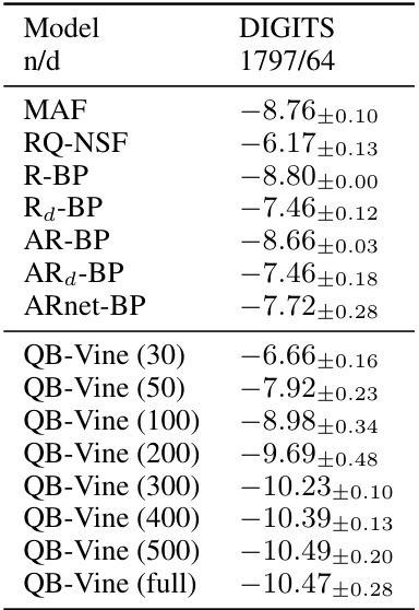
🔼 This table presents the average log predictive score (LPS) in bits per dimension (bpd) for the Digits dataset. The LPS is a metric used to evaluate the performance of density estimation models, with lower values indicating better performance. The table shows the results for various models including MAF, RQ-NSF, R-BP, AR-BP, and the QB-Vine with different training sample sizes (30, 50, 100, 200, 300, 400, 500), as well as the QB-Vine trained on the full dataset. Error bars represent standard errors over five runs.
read the caption
Table 3: Average LPS (in bpd, lower is better) over five runs with standard errors for the Digits dataset.

🔼 This table shows the average log predictive score (LPS) for various density estimation methods on five different datasets. Error bars represent two standard deviations over five runs. The QB-Vine method is compared against several other methods (KDE, DPMM, MAF, RQ-NSF, PRticle Filter, R-BP, AR-BP). The table highlights that the QB-Vine’s performance improves significantly as the dimensionality of the data increases, outperforming other methods.
read the caption
Table 1: Average log predictive score (lower is better) with error bars corresponding to two standard deviations over five runs for density estimation on datasets analysed by [35]. We note that as dimension increases, the QB-Vine outperforms all benchmarks.

🔼 This table shows the initial predictive distribution, p0, used for different datasets in the regression and classification experiments. The choice of p0, which is a hyperparameter, impacts the initialization of the Quasi-Bayesian Vine (QB-Vine) model. The table lists five datasets: BOSTON (regression), CONCR (regression), DIAB (regression), IONO (classification), and PARKIN (classification), and specifies the initial distribution (Normal or Cauchy) selected for each.
read the caption
Table 5: Choice of p0 for different regression and classification experiments.
🔼 This table presents the average log predictive scores for density estimation on several datasets. Lower scores indicate better performance. Error bars represent two standard deviations calculated over five runs for each dataset and model. The table compares the Quasi-Bayesian Vine (QB-Vine) model to several other methods, showing that QB-Vine’s performance improves relative to other methods as the dimensionality of the data increases.
read the caption
Table 1: Average log predictive score (lower is better) with error bars corresponding to two standard deviations over five runs for density estimation on datasets analysed by [35]. We note that as dimension increases, the QB-Vine outperforms all benchmarks.

🔼 This table compares the performance of the Quasi-Bayesian Vine (QB-Vine) and the Rank-ordered Normalizing Flows (RQ-NSF) models on Gaussian Mixture Models (GMMs) with varying dimensions (400, 500, 600) and five different GMMs. The Maximum Mean Discrepancy (MMD) is used as the evaluation metric, where lower values indicate better model performance. The table shows the QB-Vine consistently outperforms the RQ-NSF in all scenarios, suggesting that the QB-Vine generates samples of higher quality.
read the caption
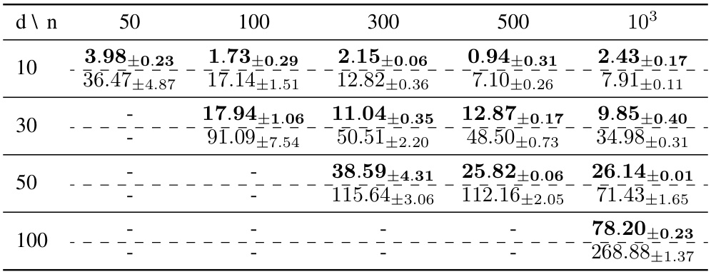
Table 7: Comparison of the MMD (lower is better) computed on samples from the QBVine and RQNSF models across different dimensions and GMMs. Each cell shows the QBVine value on top and the RQNSF value on the bottom, separated by a dotted line. The QB-Vine outperforms the RQNSF in all cases considered, demonstrating better sample quality via this metric.
Full paper#
