TL;DR#
Estimating causal effects from observational data is challenging, especially with unobserved confounding. Traditional methods often fail to identify causal quantities precisely, necessitating partial identification techniques. Neural Causal Models (NCMs) offer a promising approach, but their consistency for complex data types (continuous and categorical variables) wasn’t previously established. This raises concerns about reliable causal effect estimations using these models.
This paper tackles this challenge by demonstrating the consistency of partial identification using NCMs in a more general setting. The researchers introduce a novel representation theorem that allows for improved approximation of complex data and incorporates Lipschitz regularization during model training to ensure accuracy. Their results reveal the importance of the network architecture and the regularization method, advancing our understanding of NCMs and enhancing their reliability for causal inference tasks.
Key Takeaways#
Why does it matter?#
This paper is crucial because it establishes the consistency of neural causal models for partial identification, a significant advancement in causal inference. It addresses limitations of existing methods by expanding their applicability to continuous and categorical variables and offers practical guidelines for researchers implementing this approach. This work opens up new avenues of research by combining neural networks and causal inference for broader applications.
Visual Insights#

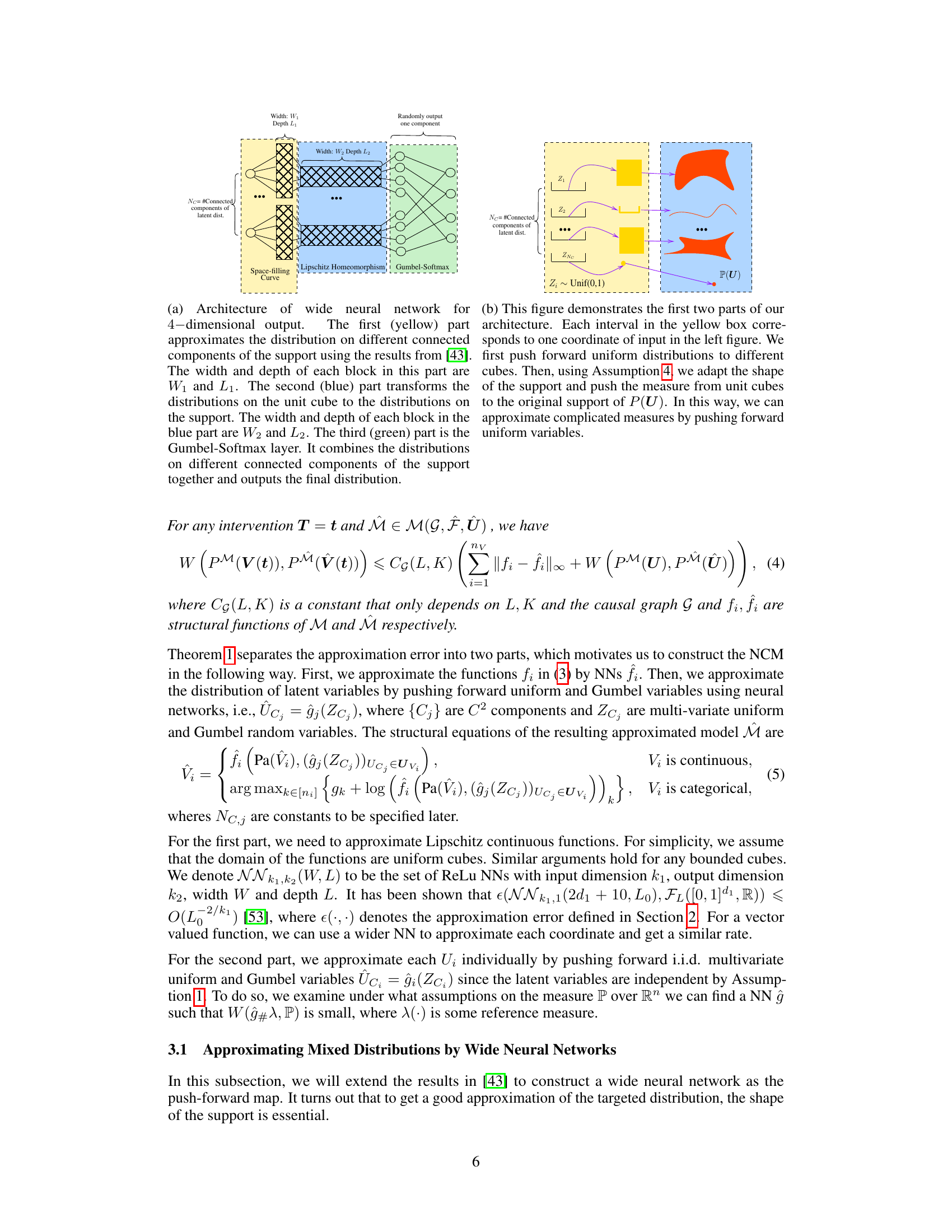
🔼 This figure shows the architecture of a neural network used to approximate probability distributions. The architecture consists of three parts: a wide neural network for approximating distributions on connected components of the support, a transformation to map distributions from unit cubes to the original support, and a Gumbel-Softmax layer to combine the distributions. The right panel illustrates how the first two parts work by showing how a uniform distribution is pushed forward through the network to approximate a more complex distribution.
read the caption
Figure 1: (a) Architecture of wide neural network for 4-dimensional output. The first (yellow) part approximates the distribution on different connected components of the support using the results from [43]. The width and depth of each block in this part are W1 and L1. The second (blue) part transforms the distributions on the unit cube to the distributions on the support. The width and depth of each block in the blue part are W2 and L2. The third (green) part is the Gumbel-Softmax layer. It combines the distributions on different connected components of the support together and outputs the final distribution. (b) This figure demonstrates the first two parts of our architecture. Each interval in the yellow box corresponds to one coordinate of input in the left figure. We first push forward uniform distributions to different cubes. Then, using Assumption 4, we adapt the shape of the support and push the measure from unit cubes to the original support of P(U). In this way, we can approximate complicated measures by pushing forward uniform variables.

🔼 This table shows the results of two experiments comparing the performance of the proposed NCM algorithm with the Autobounds algorithm for estimating average treatment effects in instrumental variable settings. The first setting uses a binary instrumental variable, while the second uses continuous variables. The table reports the average bounds and standard deviations obtained by each algorithm across multiple runs, along with the optimal bounds and the true values of the treatment effects. The results demonstrate that both algorithms generally provide bounds that cover the true values, with NCM achieving tighter bounds, particularly in the continuous setting.
read the caption
Table 1: Experiment results of 2 IV settings. The sample sizes are taken to be 5000 in each experiment. STD is the standard derivation. The experiments are repeated 10 times for binary IV and 50 times for continuous IV. In all experiments, the bounds given by both algorithms all cover the true values.
In-depth insights#
NCM Consistency Proof#
The heading ‘NCM Consistency Proof’ suggests a section dedicated to rigorously establishing the reliability of Neural Causal Models (NCMs). A core aspect would likely involve demonstrating asymptotic consistency, showing that as the amount of training data grows, the NCM’s estimations of causal effects converge to the true values. The proof would need to address challenges specific to NCMs, such as approximation errors arising from using neural networks to represent complex causal relationships and the impact of model misspecification. It would likely involve techniques from statistical learning theory, potentially using bounds on the approximation error of the NCM and analyzing sample complexity to guarantee convergence. Crucially, the proof should highlight any assumptions made about the underlying causal system (e.g., the form of causal relationships, the absence of unmeasured confounding) and their implications for the validity of the consistency result. Lipschitz continuity constraints on the network’s functions might be a key component to ensure stability and prevent overfitting, and rigorous analysis of those constraints should be incorporated. Overall, a successful ‘NCM Consistency Proof’ would greatly enhance the credibility and trustworthiness of NCMs as a causal inference tool.
SCM Approximation#
The heading ‘SCM Approximation’ suggests a crucial aspect of the research: bridging the gap between theoretical Structural Causal Models (SCMs) and their practical implementation. Approximating SCMs is essential because real-world data rarely aligns perfectly with the idealized assumptions of SCMs. The paper likely explores methods to represent SCMs using more tractable models, such as neural networks, focusing on the approximation error and its implications for causal inference. Key considerations might include the choice of approximation technique, the impact of model complexity on accuracy, and the trade-off between accuracy and computational cost. The authors probably analyze the conditions under which a reliable approximation can be achieved, potentially highlighting the limitations of certain approaches or emphasizing the need for specific regularization techniques to ensure consistency and avoid overfitting. A successful SCM approximation method would pave the way for more robust and accurate causal inference in complex, real-world scenarios. The level of detail given regarding the approximation theorems, such as error bounds and the architecture of the approximating neural networks, would be important indicators of the paper’s depth and rigor. The analysis likely touches on how well the chosen approach can handle various data types and functional forms within the SCMs.
Lipschitz Regularization#
The concept of Lipschitz regularization is crucial for ensuring the consistency of neural causal partial identification. Without Lipschitz regularization, the neural network’s approximation may not be asymptotically consistent, leading to inaccurate partial identification bounds. This is because the approximation error can grow arbitrarily large without such constraints. Lipschitz continuity ensures that the network’s outputs do not change drastically with small changes in the input, promoting stability and robustness. The paper emphasizes this via counterexamples demonstrating how failure to enforce Lipschitz continuity can lead to inconsistencies. Formal consistency proofs are presented only after incorporating Lipschitz regularization techniques, which limit the gradient magnitude during training. This restriction enhances the reliability of the resulting architectures by bounding the impact of approximation error on the partial identification bounds, ultimately leading to more accurate and trustworthy causal inferences.
Partial ID via NCMs#
The heading “Partial ID via NCMs” suggests a method for partial identification of causal effects using neural causal models (NCMs). Partial identification acknowledges the limitations of observational data in fully specifying causal relationships, especially when unobserved confounding exists. NCMs, leveraging neural networks, offer a potentially powerful approach to this problem. The core idea is to train a neural network to represent the observed data distribution while respecting the constraints imposed by a known causal graph. By exploring the range of possible causal models consistent with the observed data, the NCM framework can provide bounds on the target causal quantity, thus addressing the partial identification challenge. This approach contrasts with traditional methods that may rely on restrictive assumptions or specific identification strategies, making NCMs a flexible and potentially more powerful technique. A key area of investigation would likely focus on the consistency and efficiency of NCM-based partial identification, exploring factors such as network architecture, training methods, and sample size. The effectiveness of this approach could hinge on the capacity of NCMs to effectively approximate the complex probability distributions underlying the observed data and the chosen causal model.
Future Directions#
Future research could explore relaxing the Lipschitz constraint in neural causal models, allowing for greater model flexibility and potentially improved accuracy. Investigating alternative architectures beyond those presented, such as using deep networks more extensively, could enhance model capacity and approximation capabilities. Another critical area is developing techniques for handling high-dimensional data more effectively, as current methods can struggle with high-dimensionality. Addressing the computational cost of the optimization procedure is also important, as current methods can be computationally intensive, especially for large datasets. Finally, expanding the theoretical framework to encompass a broader range of causal structures and handling scenarios with more complex confounding is a significant challenge for future work.
More visual insights#
More on figures
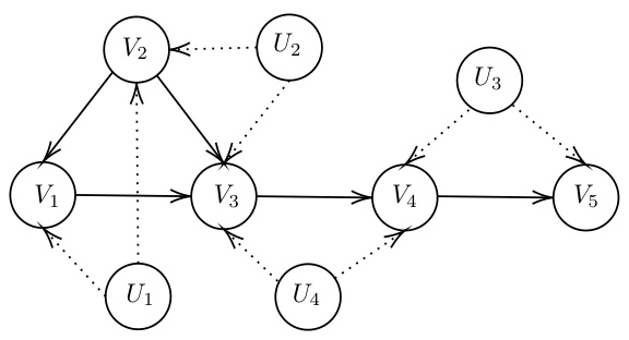
🔼 This figure shows a simple example of a structural causal model (SCM). The circles represent variables, and the arrows indicate causal relationships between them. The solid arrows denote direct causal effects, while the dotted arrows show the presence of unobserved confounders (latent variables U1-U4) influencing multiple observed variables. This model demonstrates a complex causal structure with both direct and indirect effects and unobserved confounding that requires more sophisticated methods for causal inference.
read the caption
Figure 2: An SCM example.
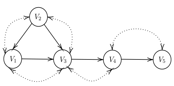
🔼 This figure shows a causal graph representing a structural causal model (SCM). The nodes represent variables, and the arrows indicate the direction of causality. The graph is used as an example within the paper to illustrate concepts related to causal inference and the construction of neural causal models (NCMs). Specifically, it demonstrates a setting where variables may be influenced by shared latent variables (represented by bi-directed edges), highlighting the complexity of causal relationships which neural methods aim to approximate.
read the caption
Figure 3: The causal graph of this SCM.
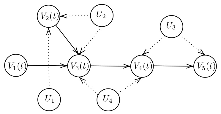
🔼 This figure shows the structural causal model (SCM) after applying an intervention on variable V₁. The intervention sets V₁ to a specific value, denoted as ’t’. The resulting graph shows how the other variables V₂, V₃, V₄, and V₅ are affected by this intervention, taking into account the causal relationships between them and the latent variables U₁, U₂, U₃, and U₄. The dotted lines indicate the presence of unobserved confounding, signifying correlations between certain latent variables that influence the observed variables.
read the caption
Figure 4: The SCM after intervention V₁ = t.
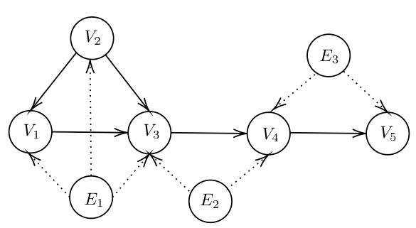
🔼 This figure is a causal graph showing the relationships between variables V1, V2, V3, V4, V5, and latent variables E1, E2, E3 in a structural causal model (SCM). Arrows represent direct causal influences; for instance, V2 causally influences V1 and V3. The dotted lines indicate the presence of unobserved confounders; for example, E1 confounds V1 and V2. The graph illustrates the complex dependencies and confounding present in the SCM, essential for understanding the challenges of causal inference in this context.
read the caption
Figure 3: The causal graph of this SCM.
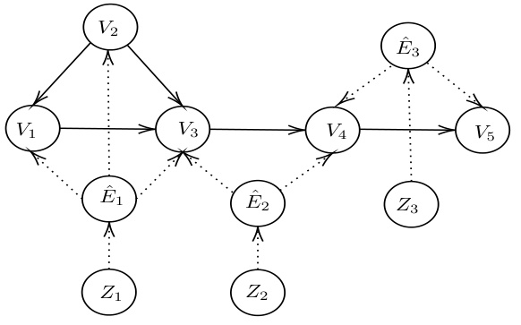
🔼 This figure shows the canonical representation of the causal graph shown in Figure 3. The canonical representation simplifies the SCM by using only one latent variable for each C2-component of the graph. This is done by merging the original latent variables to create new latent variables, each associated with a C2-component. This representation is useful for approximating the SCM using neural networks, as each C2-component can be treated independently.
read the caption
Figure 5: The canonical representation of Figure 3.
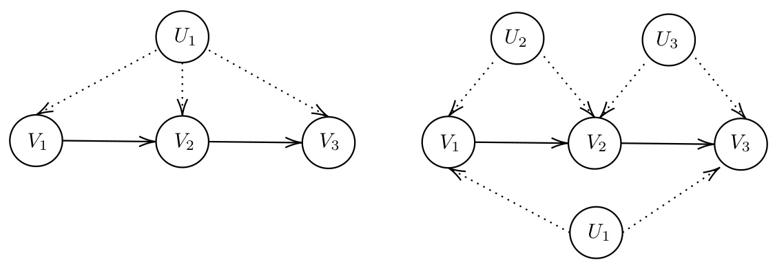
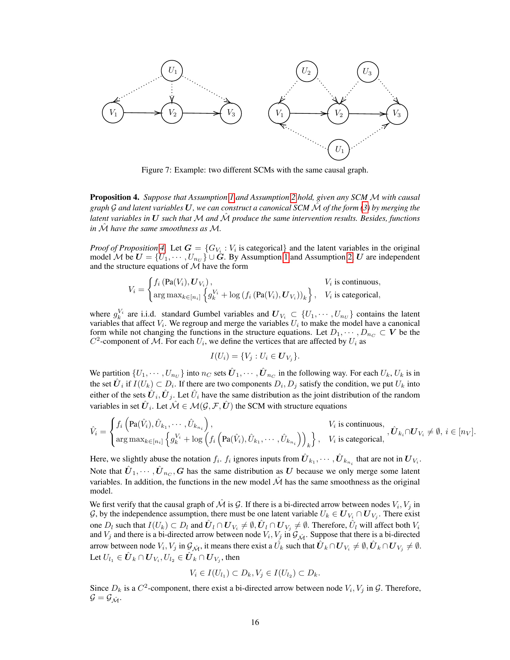
🔼 This figure shows two different structural causal models (SCMs) that share the same causal graph. The left panel depicts an SCM where a single latent variable, U1, influences V1, V2, and V3. The right panel displays an SCM where there are three latent variables (U1, U2, U3). U2 and U3 each independently influence V2 and V3 while U1 influences all three variables. The figure highlights that multiple SCMs can generate the same observational data distribution, even if they have different underlying causal structures and latent variable configurations.
read the caption
Figure 7: Example: two different SCMs with the same causal graph.
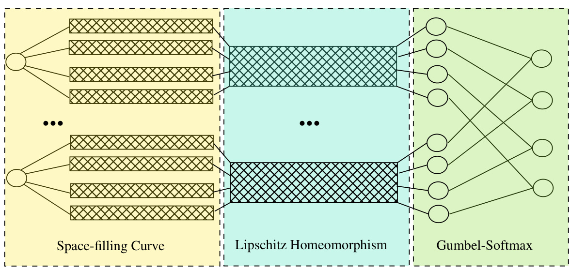
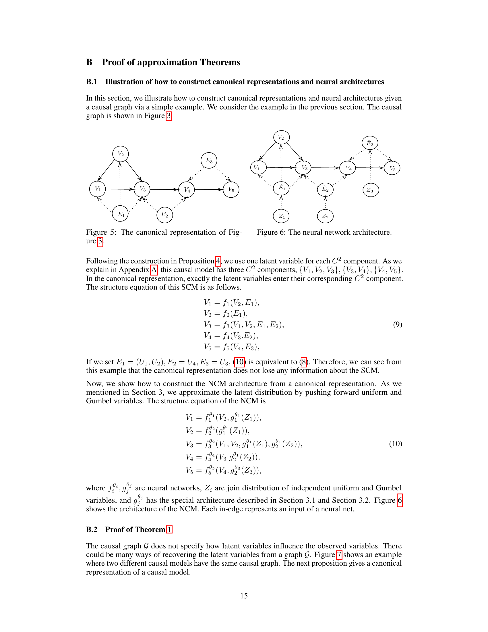
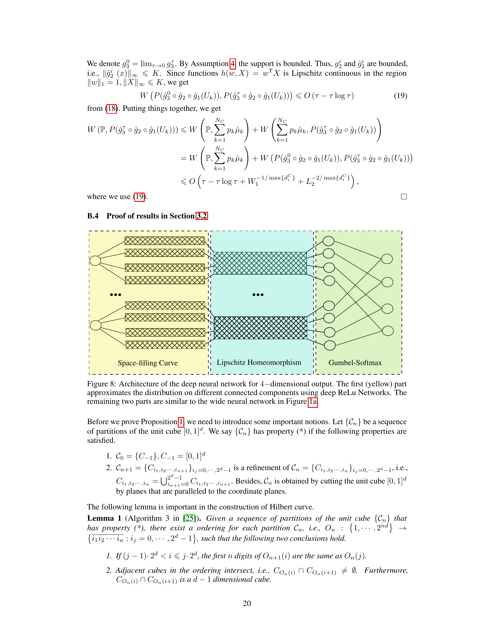
🔼 This figure illustrates the architecture of a wide neural network used to approximate a probability distribution. It’s composed of three main parts: a space-filling curve component (yellow), a Lipschitz homeomorphism component (light blue), and a Gumbel-Softmax layer (light green). The space-filling curve part approximates the distribution across different connected components of the support. The Lipschitz homeomorphism part transforms the distributions into the original support. Finally, the Gumbel-Softmax layer combines these distributions to provide the final output distribution.
read the caption
Figure 1: Architecture of wide neural network for 4-dimensional output. The first (yellow) part approximates the distribution on different connected components of the support using the results from [43]. The width and depth of each block in this part are W1 and L1. The second (blue) part transforms the distributions on the unit cube to the distributions on the support. The width and depth of each block in the blue part are W2 and L2. The third (green) part is the Gumbel-Softmax layer. It combines the distributions on different connected components of the support together and outputs the final distribution.
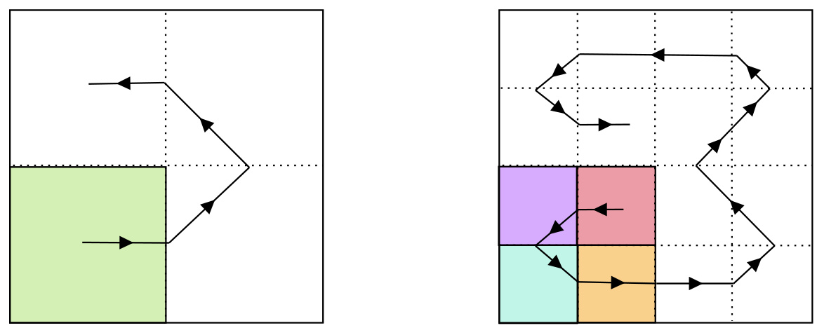
🔼 This figure illustrates the construction of the Hilbert space-filling curve used in the proof of Proposition 1. The left panel shows the first two steps of the iterative process, subdividing the unit square into smaller squares and tracing a continuous curve through them. The colors represent the order in which squares are visited by the curve. The right panel shows a more advanced stage of this iterative process, illustrating how the curve fills the space. The method adjusts the speed of the curve to match the target probability distribution P (the original distribution in Proposition 1) over the unit square, ultimately demonstrating that any distribution satisfying Assumption 5 can be represented as the push-forward of the Lebesgue measure on [0,1] by a Hölder continuous curve.
read the caption
Figure 9: The construction of Hilbert curve.
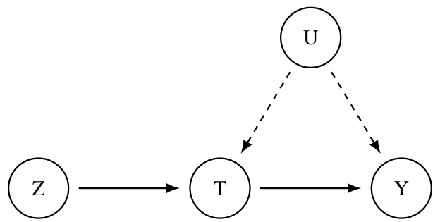
🔼 This figure shows a causal graph representing an instrumental variable model. Z is the instrumental variable, which affects the treatment variable T, but not the outcome variable Y directly. T in turn influences Y. There is also an unobserved confounder, U, affecting both T and Y, indicating a confounding effect that needs to be accounted for. This structure is common in causal inference scenarios where direct observation of the causal relationship between T and Y is confounded. The instrumental variable Z allows us to overcome the confounding effect by exploiting its independent relationship with T and its effect on the outcome variable only through T.
read the caption
Figure 10: Instrumental Variable (IV) graph. Z is the instrumental variable, T is the treatment and Y is the outcome.
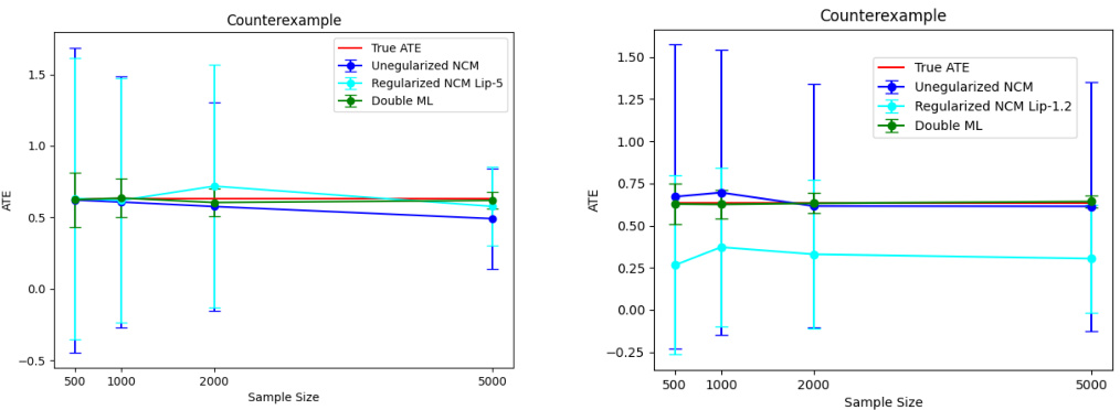
🔼 This figure compares the performance of Lipschitz regularized and unregularized neural causal algorithms for estimating average treatment effects (ATEs). Two different neural network architectures are used, one with medium size (width 128, depth 3) and another with small size (width 3, depth 1). For both architectures, the projected gradient method is employed for Lipschitz regularization. The results are shown for various sample sizes, representing the average upper and lower bounds obtained from 5 repetitions for each size. The goal is to illustrate how Lipschitz regularization affects the accuracy and consistency of ATE estimation using neural causal models.
read the caption
Figure 11: Comparison of Lipschitz regularized and unregularized neural causal algorithm. The two figures show the results of different architectures. The figure on the left side uses a medium-sized NN (width 128, depth 3) to approximate each structural function, while the right figure uses extremely small NNs (width 3, depth 1). In all experiments, we use the projected gradient to regularize the weight of the neural network. For each sample size, we repeat the experiment 5 times and take the average of the upper (lower) bound.
More on tables

🔼 This table compares the performance of the proposed Neural Causal Model (NCM) approach against the Autobounds algorithm for two different instrumental variable (IV) settings: a binary IV setting and a continuous IV setting. For each setting, it shows the average bound, standard deviation of the length of the bound, the optimal bound (obtained using linear programming for binary IV and not available for continuous IV), and the true value of the causal quantity. The sample size is 5000 in all experiments, and the experiments were repeated multiple times to obtain statistically reliable estimates.
read the caption
Table 1: Experiment results of 2 IV settings. The sample sizes are taken to be 5000 in each experiment. STD is the standard derivation. The experiments are repeated 10 times for binary IV and 50 times for continuous IV. In all experiments, the bounds given by both algorithms all cover the true values.

🔼 This table compares the performance of the proposed Neural Causal Model (NCM) approach with the Autobounds algorithm [14] on two instrumental variable (IV) settings: one with binary variables and one with continuous variables. The table shows the average bounds obtained by each algorithm, the standard deviation of the bound lengths, the success rate of the algorithms in covering the true value (which was known in these experiments), and the true values themselves. The sample sizes are consistent at 5000 across all experiments. Note that the NCM approach shows slightly tighter bounds than the Autobounds method.
read the caption
Table 1: Experiment results of 2 IV settings. The sample sizes are taken to be 5000 in each experiment. STD is the standard derivation. The experiments are repeated 10 times for binary IV and 50 times for continuous IV. In all experiments, the bounds given by both algorithms all cover the true values.
Full paper#

