TL;DR#
Many machine learning models lack transparency, making it difficult to understand how decisions are made. Existing methods for explaining model decisions often result in complex and unintuitive explanations. The concept of global sparsity, focusing on the overall model complexity, is not always relevant for individuals affected by model decisions. Local sparsity, also known as decision sparsity, matters more, but it is challenging to quantify and optimize. This paper tackles this problem by extending the Sparse Explanation Value (SEV) framework.
This work introduces cluster-based SEV and tree-based SEV, which improve explanation closeness and credibility. A new method to improve the credibility of explanations is also presented, along with algorithms to optimize decision sparsity during model training. The findings demonstrate that the proposed SEV variants achieve better sparsity, closeness, and credibility compared to existing counterfactual explanation techniques, making AI models more understandable and trustworthy.
Key Takeaways#
Why does it matter?#
This paper is crucial for researchers working on interpretable machine learning, especially those focused on decision-making models. It introduces novel methods for optimizing decision sparsity, leading to more meaningful and credible explanations which is a highly relevant topic in today’s AI research. The proposed algorithms and theoretical framework provide valuable tools for building more transparent and understandable AI systems.
Visual Insights#

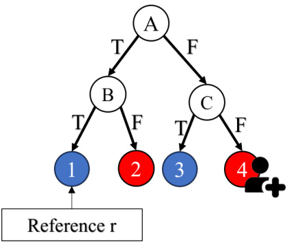
🔼 This figure illustrates a SEV hypercube with 2³ = 8 vertices for a model f, an instance xᵢ with label f(xᵢ) = 1, and a reference r. Each vertex is a Boolean vector that represents different alignment combinations (setting features to the reference or not). Vertices are adjacent when their Boolean vectors differ in one bit. The score of vertex v is f(xv), indicating if the modified instance is positive (1) or negative (0). The shortest path from a query (positive instance) to a negative vertex represents the SEV.
read the caption
Figure 1: SEV Hypercube

🔼 This table shows an example of how different methods for calculating Sparse Explanation Values (SEV) produce different explanations for the same query point in the FICO dataset. It compares four SEV variations: SEV¹, which uses a single reference point (the population mean); SEV®, which uses cluster-based references; SEVF, which uses flexible references; and SEVT, which uses tree-based references. The table highlights the resulting explanation’s sparsity (number of features changed) for each method.
read the caption
Table 1: An example for a query in the FICO Dataset with different kinds of explanations, SEV¹ represents the SEV calculation with one single reference using population mean, SEV® represents the cluster-based SEV, SEVF represents the flexible-based SEV. SEVT represents the tree-based SEV The columns are four features.
In-depth insights#
Decision Sparsity#
Decision sparsity, a crucial concept in machine learning interpretability, focuses on minimizing the amount of information necessary to explain an individual prediction. Unlike global sparsity metrics, which consider the overall model complexity, decision sparsity centers on the specific features impacting a single decision. This local perspective is particularly important when dealing with models where individuals are subject to the model’s output, as they are less concerned with the global model’s structure and more interested in understanding why a specific decision was made concerning them. The Sparse Explanation Value (SEV) is a key metric for measuring decision sparsity, focusing on the minimum number of feature changes needed to alter the prediction. However, SEV’s utility can be enhanced by incorporating considerations of credibility and closeness, ensuring that the explanation is not only sparse but also realistic and intuitive. The research explores various refinements to SEV such as cluster-based and tree-based approaches to optimize for these criteria, resulting in more meaningful and trustworthy explanations.
SEV Enhancements#
The core concept revolves around enhancing the Sparse Explanation Value (SEV) framework for improved model interpretability. Key enhancements focus on addressing the limitations of the original SEV definition, which relied on a single, potentially distant, reference point. The proposed solutions introduce cluster-based SEV, using multiple reference points to improve explanation closeness and credibility. A further refinement is tree-based SEV, which leverages the structure of decision trees for computationally efficient and intuitive explanations. Flexibility in choosing reference points is also incorporated to further optimize sparsity and allow for fine-tuning of explanations. By incorporating these improvements, SEV is significantly enhanced to produce more meaningful, credible, and locally sparse explanations vital for interpretable machine learning models, thereby improving human understanding and trust.
Model Optimization#
The model optimization section of this research paper is crucial because it directly addresses how to improve the model’s ability to produce sparse and credible explanations. The authors recognize that merely calculating Sparse Explanation Value (SEV) isn’t sufficient; they need models inherently biased towards generating such explanations. Two key approaches are presented: gradient-based optimization, using a differentiable loss function to penalize high-SEV instances, and search-based optimization, leveraging the Rashomon set of equally performing models to identify the sparsest one. The gradient-based method offers efficiency but may not guarantee global optimality. Conversely, the search-based approach ensures optimal SEV but is computationally more expensive. This trade-off highlights a central challenge in interpretable machine learning: the tension between efficient model training and the generation of truly optimal, sparse explanations. The success of both strategies underscores the potential of directly integrating sparsity into the model training process, moving beyond post-hoc explanation methods. This focus on model-level changes rather than post-hoc modifications is a significant contribution, suggesting a shift towards models that prioritize both accurate prediction and inherently interpretable outputs.
Tree-Based SEV#
The proposed “Tree-Based SEV” method offers a computationally efficient and insightful approach to calculating Sparse Explanation Values (SEV). Leveraging the inherent tree structure of a decision tree model, it identifies the shortest path from a positive prediction (the query point) to a negative leaf node, representing the reference point for the opposite class. This path directly translates to the minimal set of feature changes needed to alter the prediction, providing a sparse and locally meaningful explanation. The method elegantly incorporates the concept of closeness and credibility, as the reference point is naturally situated within the high-density region of the opposite class in feature space. This approach significantly improves efficiency over standard SEV calculations, particularly in high-dimensional datasets, by avoiding exhaustive searches across the hypercube. The theoretical guarantees associated with this method further enhance its value and reliability, ensuring that the resulting explanations are provably optimal in terms of sparsity and distance. The effectiveness of Tree-Based SEV is demonstrated experimentally, showcasing its ability to deliver superior explanations characterized by both high sparsity and credibility.
Future Work#
Future research could explore extending the Sparse Explanation Value (SEV) framework to handle more complex scenarios, such as multi-class classification and non-binary outcomes. Investigating the impact of different clustering algorithms and reference point selection methods on SEV calculations would further enhance the robustness and explainability of the approach. Addressing the computational cost associated with calculating SEV for large datasets and high-dimensional data is crucial for practical applications. Finally, a more rigorous theoretical analysis of SEV’s properties, particularly its connection to causal inference, could deepen our understanding of its strengths and limitations. Developing efficient algorithms to optimize model parameters directly for SEV sparsity without sacrificing predictive accuracy warrants further study, including the exploration of different loss functions and optimization techniques. Further investigation into the credability of SEV explanations is needed, potentially by incorporating measures of uncertainty and developing methods to assess how representative the generated explanations are of the true underlying data distribution.
More visual insights#
More on figures
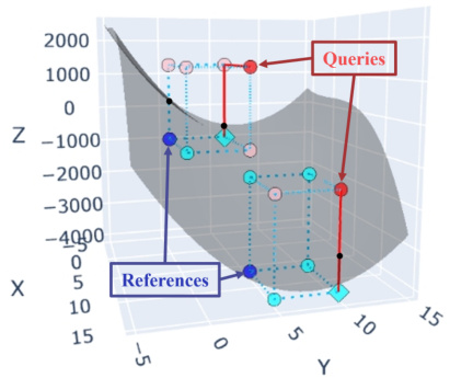
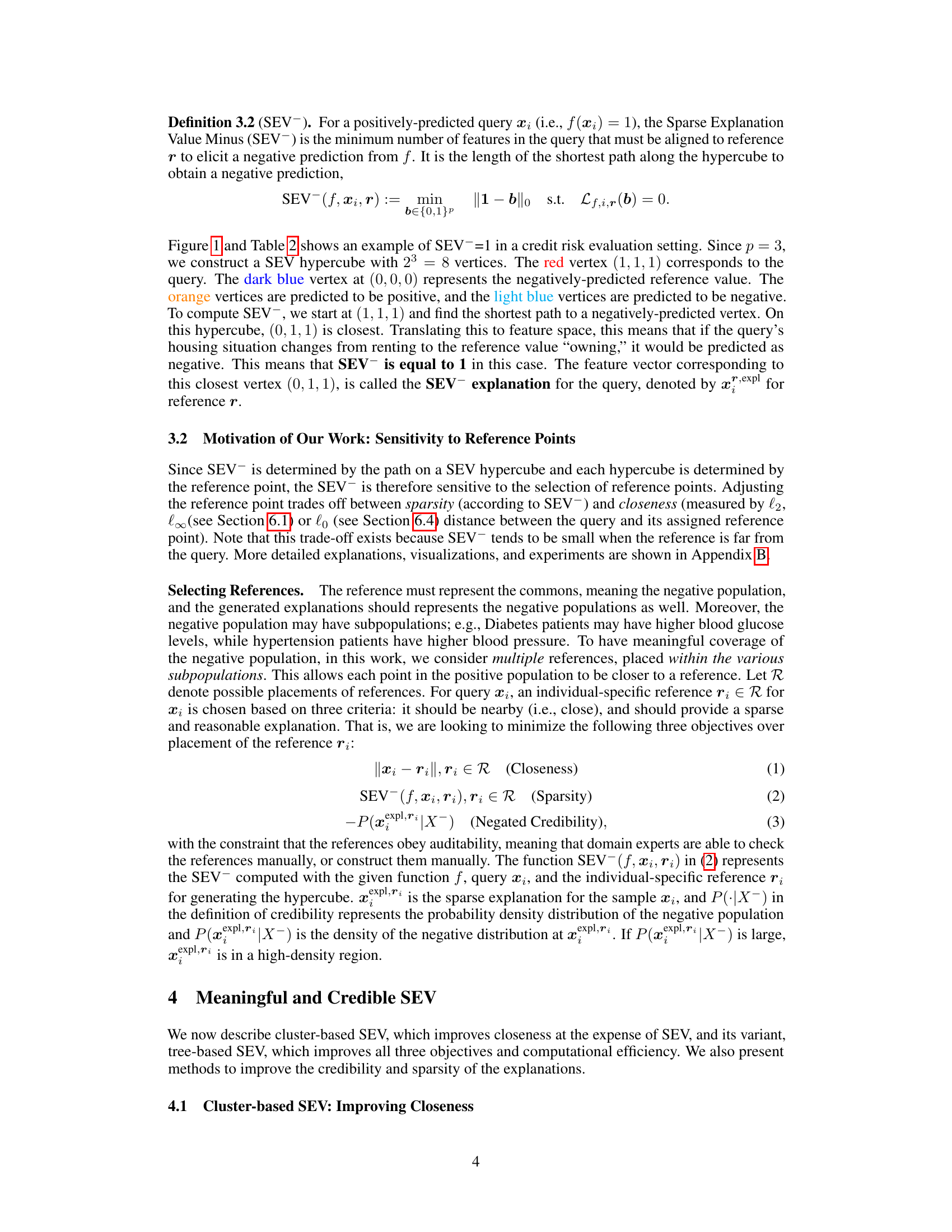
🔼 This figure illustrates the calculation of cluster-based SEV (SEV©) for two examples. Each red dot represents a query, while each blue dot represents a reference. For each instance, the closest centroid is selected and the SEV hypercube is considered. Cyan points represent negatively predicted vertices and pink points represent positively predicted vertices. Following the red lines, the SEV© for the two queries are 2 and 1, respectively.
read the caption
Figure 2: Cluster-based SEV
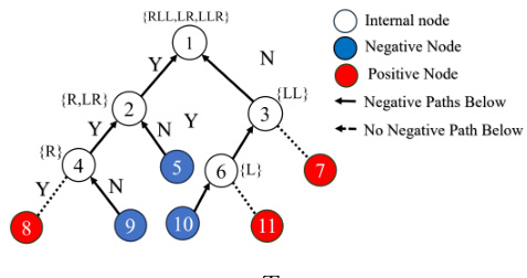
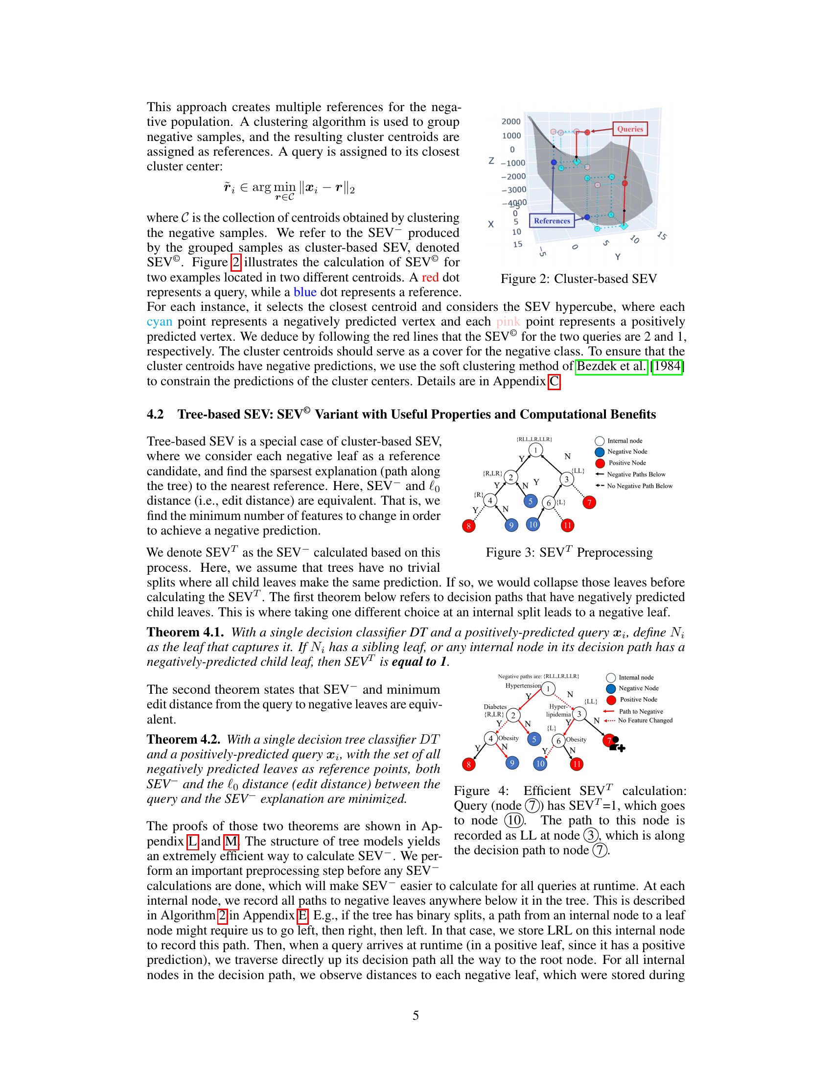
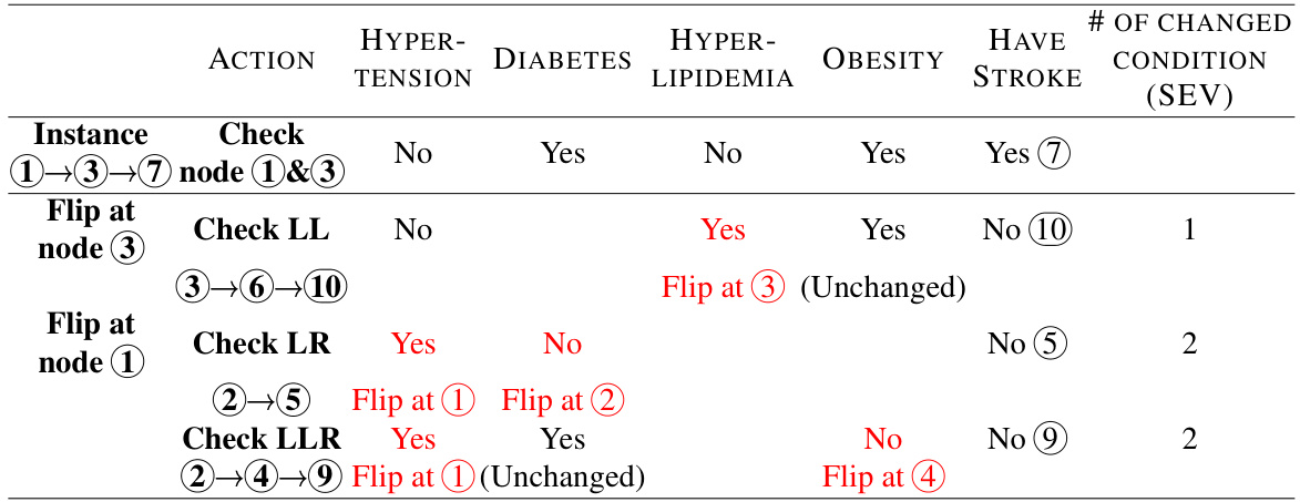
🔼 This figure illustrates the preprocessing step for tree-based SEV (SEVT) calculations. It shows how negatively predicted leaf nodes are identified and their paths recorded at internal nodes. This preprocessing speeds up SEVT calculation at runtime by allowing the algorithm to quickly identify relevant paths to negative leaves from the query point in the tree. The figure uses color-coding to represent different node types (internal, negative, positive) and arrows to represent the path from each internal node to negatively predicted leaves. The path information (e.g., RLL, LR, LLR) is recorded at each internal node to represent a sequence of decisions to reach negatively predicted leaves. This allows the algorithm to avoid redundant calculations during runtime.
read the caption
Figure 3: SEVT Preprocessing

🔼 This figure illustrates the preprocessing step for calculating tree-based SEV (SEVT). It shows how to efficiently find the shortest paths from a positively-predicted query point to negatively-predicted leaf nodes in a decision tree. The preprocessing step involves identifying all paths leading to negative leaves from each internal node in the tree and storing those paths for later use. During SEVT calculation, the algorithm only needs to traverse upward from the query leaf node, checking the pre-computed negative paths at each internal node. This significantly speeds up the SEVT calculation compared to calculating SEV from scratch.
read the caption
Figure 3: SEVT Preprocessing

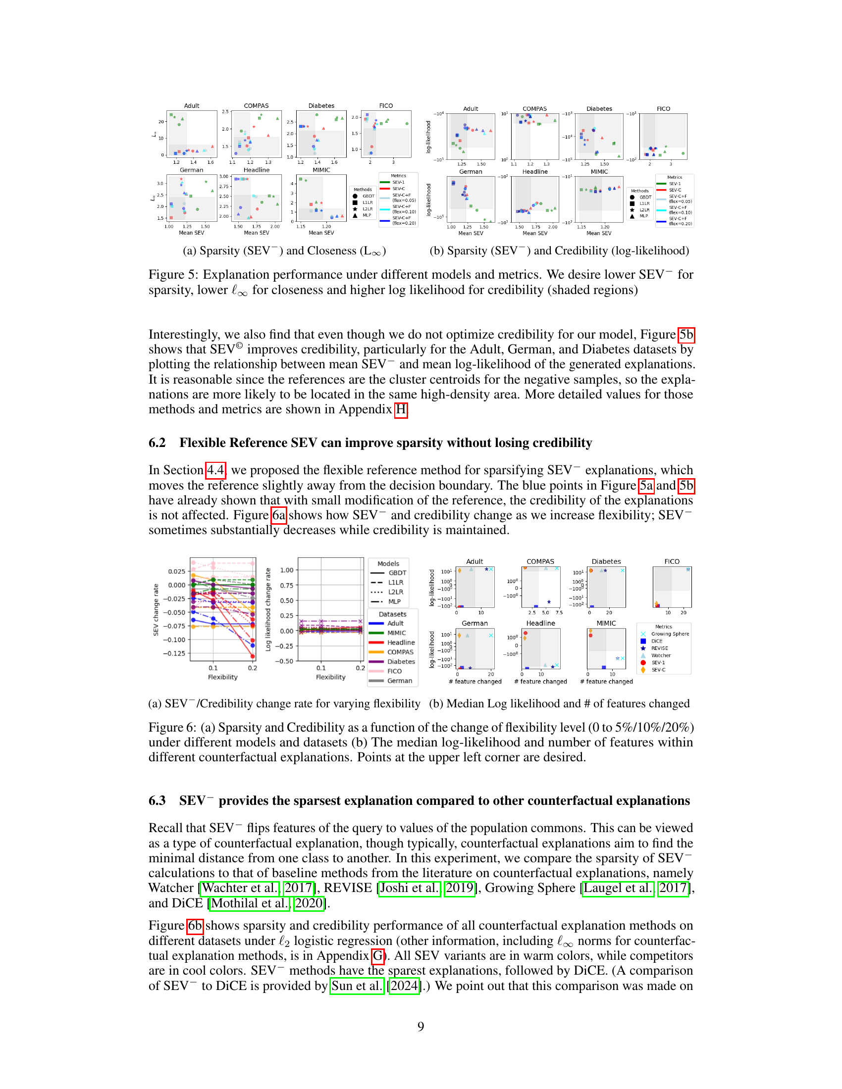
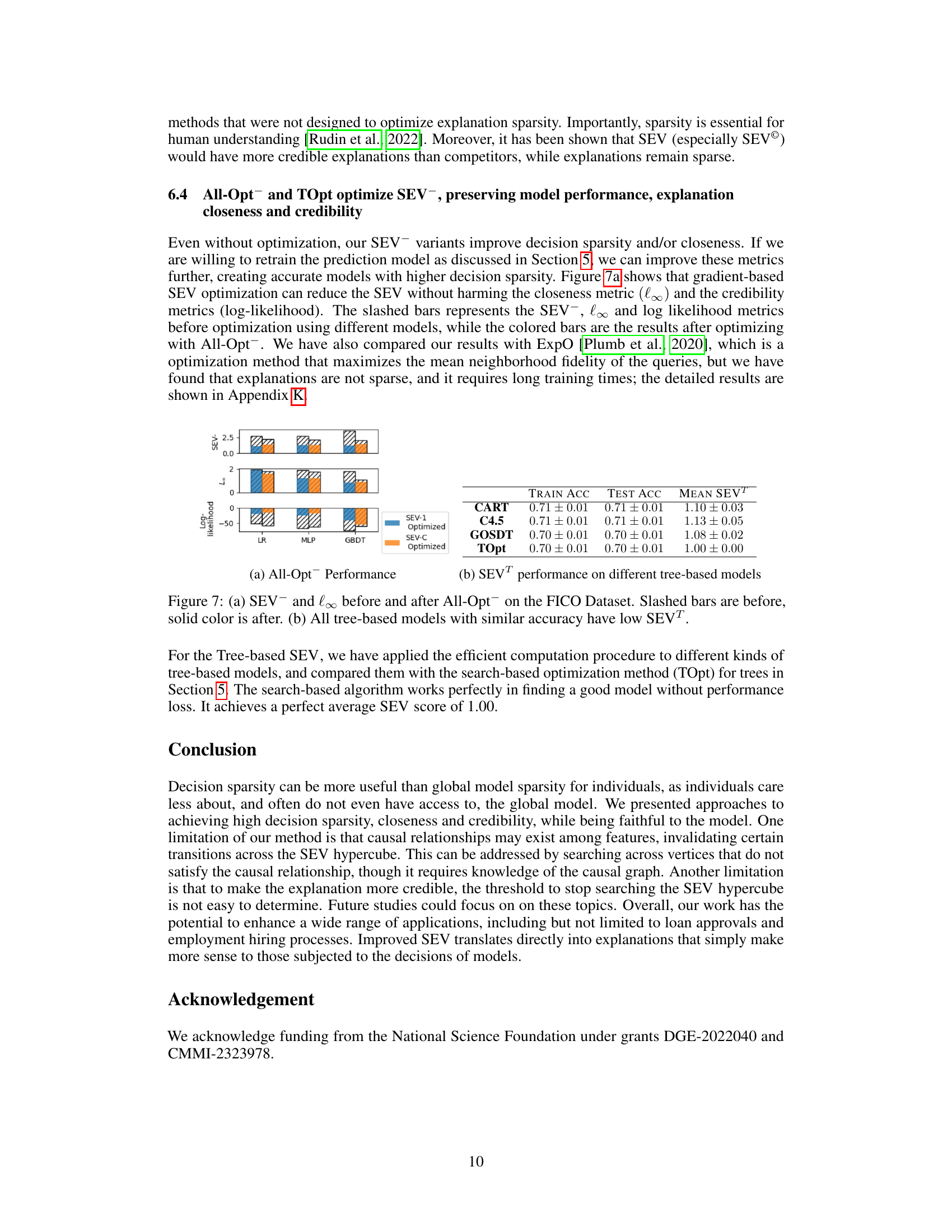
🔼 This figure compares the performance of different SEV variants (SEV¹, SEV©, and SEV©+F) across multiple datasets and model types. The left panel shows the trade-off between sparsity (measured by SEV¯) and closeness (measured by the L∞ distance between the query and its explanation). The right panel illustrates the relationship between sparsity and credibility, where higher log-likelihood indicates better credibility. The shaded regions in both plots highlight the desired areas of high credibility, low SEV¯ (high sparsity) and low L∞ (high closeness). The results suggest that SEV© generally improves both closeness and credibility compared to SEV¹, while SEV©+F offers a way to further improve sparsity by adjusting the reference point.
read the caption
Figure 5: Explanation performance under different models and metrics. We desire lower SEV¯ for sparsity, lower l∞ for closeness and higher log likelihood for credibility (shaded regions)

🔼 This figure compares the performance of different SEV variants (SEV¹, SEV©, SEV©+F) across various datasets and machine learning models. It visualizes the trade-offs between three key aspects of model explanations: sparsity (measured by SEV, lower is better), closeness (measured by l∞ distance between the query and explanation, lower is better), and credibility (measured by log-likelihood of the explanation within the negative class distribution, higher is better). The shaded regions in the plots highlight the desirable areas with low SEV¯, low l∞, and high log-likelihood.
read the caption
Figure 5: Explanation performance under different models and metrics. We desire lower SEV¯ for sparsity, lower l∞ for closeness and higher log likelihood for credibility (shaded regions)

🔼 This figure compares the performance of different SEV variants (SEV¹, SEV©, and SEV©+F) across multiple datasets and models. It visualizes the trade-off between sparsity (SEV¯), closeness (l∞), and credibility (log-likelihood). Lower SEV¯ values indicate sparser explanations, while lower l∞ values represent closer explanations to the original data point. Higher log-likelihood values signify higher credibility. The shaded regions in the plots highlight the desired area of optimal performance: low SEV¯, low l∞, and high log-likelihood.
read the caption
Figure 5: Explanation performance under different models and metrics. We desire lower SEV¯ for sparsity, lower l∞ for closeness and higher log likelihood for credibility (shaded regions)

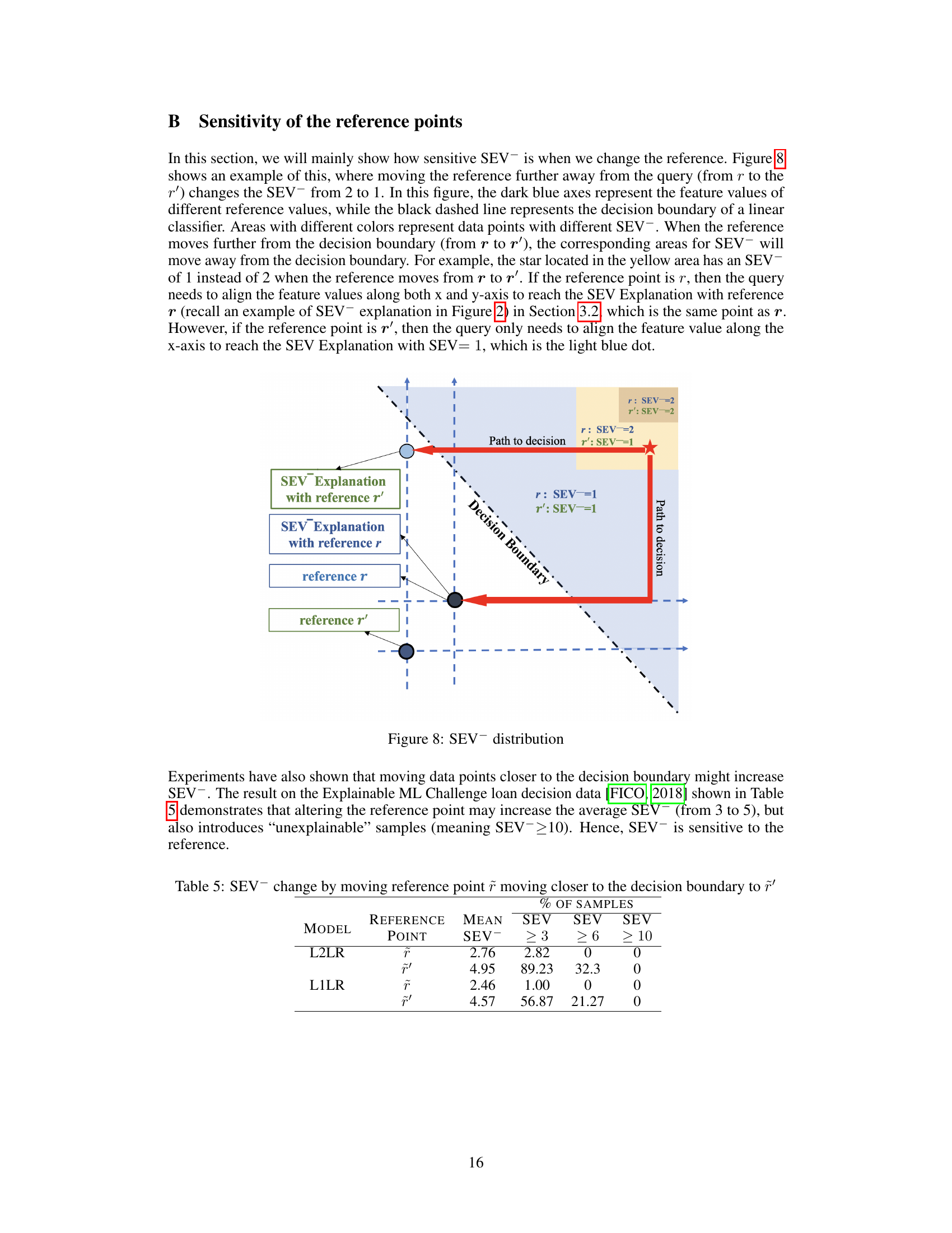
🔼 This figure demonstrates the sensitivity of SEV to the choice of reference points. Moving the reference point further away from the query (from r to r’) changes the SEV from 2 to 1. The figure shows how the areas with different SEV values move as the reference point changes. Specifically, it illustrates how moving the reference point away from the decision boundary causes the SEV values to also move away from the decision boundary. This indicates that the sparsity of the explanations is sensitive to the location of the reference point.
read the caption
Figure 8: SEV distribution

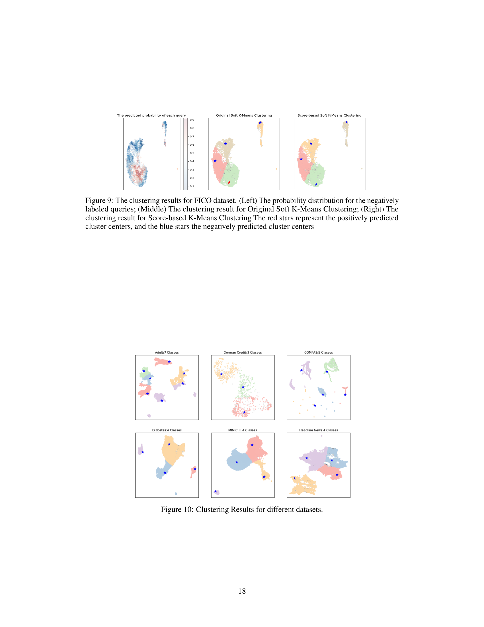
🔼 This figure compares the clustering results of three different methods on the FICO dataset. The leftmost panel shows the probability distribution of negative samples. The middle panel shows the clustering result using original soft k-means, and the rightmost panel shows the result from score-based soft k-means. The red stars represent positively predicted cluster centers, while the blue stars represent negatively predicted cluster centers. The score-based soft k-means method aims to penalize positive clusters to ensure that the generated cluster centers are all negatively predicted, hence resulting in a more effective SEV calculation.
read the caption
Figure 9: The clustering results for FICO dataset. (Left) The probability distribution for the negatively labeled queries; (Middle) The clustering result for Original Soft K-Means Clustering; (Right) The clustering result for Score-based K-Means Clustering The red stars represent the positively predicted cluster centers, and the blue stars the negatively predicted cluster centers

🔼 This figure visualizes the results of the clustering algorithm applied to six different datasets used in the paper. Each subplot represents a dataset, showing the clusters formed by the algorithm. The points in each subplot represent individual data points in that dataset, colored according to the cluster they belong to. Blue stars mark the cluster centers, which are used as reference points in the SEV calculation. The datasets included are: Adult, German Credit, COMPAS, Diabetes, MIMIC III, and Headline News. The number of clusters for each dataset is indicated in the title of each subplot.
read the caption
Figure 10: Clustering Results for different datasets.
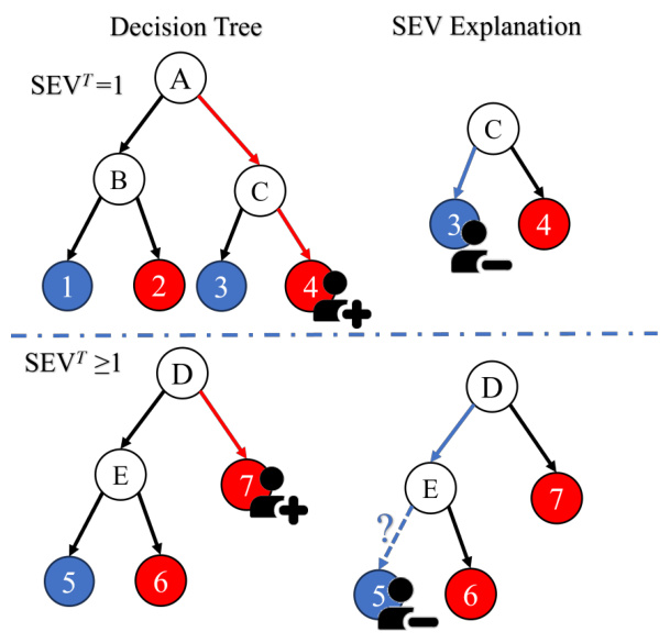
🔼 This figure illustrates Theorem 4.1, which states that if a positively predicted query node in a decision tree has a sibling leaf node or an ancestor node with a negatively predicted child leaf node, the tree-based SEV (SEVT) is equal to 1. The left side shows two example decision trees. In the top tree, the query node (red) has a sibling (blue), so changing one feature leads to a negative prediction (SEVT=1). The bottom tree shows a case where the query node does not have a sibling leaf node, but an ancestor node has a negatively predicted child node, so again, changing one feature leads to a negative prediction (SEVT=1). The right side shows the corresponding SEV explanations; the red arrows indicate the changes necessary to achieve a negative prediction. The dashed line separates the two cases.
read the caption
Figure 11: Example of SEVT=1 in Theorem 4.1
🔼 This figure provides an example to illustrate Theorem 4.1, which states that if a positively predicted query’s leaf node has a sibling leaf node, or any internal node in its decision path has a negatively predicted child leaf, then the Tree-based Sparse Explanation Value (SEVT) is equal to 1. The figure shows two decision trees. The left tree shows a complete decision tree where nodes 1 and 3 are negatively predicted leaves, while node 2 and 4 are positively predicted leaves. The right tree shows the subtree relevant to the explanation, containing only nodes that directly affect the decision for the given instance represented by a person icon with a plus sign. A single change is sufficient to reach a negatively predicted leaf, resulting in SEVT = 1. Conversely, if a positively-predicted query’s leaf has no sibling leaf and there are no internal nodes with negatively-predicted child nodes, SEVT would be greater than 1, which the theorem states, and is illustrated.
read the caption
Figure 11: Example of SEVT=1 in Theorem 4.1
More on tables

🔼 This table demonstrates an example of how different SEV methods (SEV¹, SEV®, SEVF, SEVT) generate explanations for a single query point in the FICO dataset. It shows how the choice of reference point and method impacts the sparsity of the explanation (number of features changed) and its overall credibility. SEV¹ uses the population mean as the reference; SEV® uses cluster centroids; SEVF allows for flexibility in the reference point; and SEVT uses the leaf nodes of a decision tree.
read the caption
Table 1: An example for a query in the FICO Dataset with different kinds of explanations, SEV¹ represents the SEV calculation with one single reference using population mean, SEV® represents the cluster-based SEV, SEVF represents the flexible-based SEV. SEVT represents the tree-based SEV The columns are four features.
🔼 This table shows an example of how different SEV methods (SEV¹, SEV®, SEVF, SEVT) generate explanations for a single query in the FICO dataset. SEV¹ uses a single reference point (the population mean). SEV® uses multiple reference points, one for each cluster in the data. SEVF is similar to SEV® but allows for slight adjustments to the reference points to improve sparsity. SEVT uses a decision tree model to calculate SEV. The table shows the changes in feature values that lead to a change in prediction for each method, highlighting the differences in sparsity and the locations of the resulting counterfactual instances.
read the caption
Table 1: An example for a query in the FICO Dataset with different kinds of explanations, SEV¹ represents the SEV calculation with one single reference using population mean, SEV® represents the cluster-based SEV, SEVF represents the flexible-based SEV. SEVT represents the tree-based SEV The columns are four features.

🔼 This table presents a comparison of four different methods for calculating Sparse Explanation Values (SEV) for a single query in the FICO dataset. The methods compared are: * SEV¹: Uses a single reference point calculated as the population mean. * SEV®: Uses multiple reference points, one for each cluster in the negative class. * SEVF: Uses a flexible reference point, allowing for slight adjustments to improve sparsity. * SEVT: Uses a tree-based approach, placing a reference point on each negative leaf node. For each method, the table shows the resulting SEV, along with the four features that were changed to achieve the different explanation values. The purpose is to illustrate how different approaches to defining and calculating SEV yield explanations that vary in sparsity and closeness to the original query point.
read the caption
Table 1: An example for a query in the FICO Dataset with different kinds of explanations, SEV¹ represents the SEV calculation with one single reference using population mean, SEV® represents the cluster-based SEV, SEVF represents the flexible-based SEV. SEVT represents the tree-based SEV The columns are four features.

🔼 This table demonstrates the application of four different SEV (Sparse Explanation Value) calculation methods on a single query from the FICO dataset. It shows how different methods - standard SEV using a single reference point (SEV¹), cluster-based SEV (SEV©), flexible-reference SEV (SEVF), and tree-based SEV (SEVT) - result in varying numbers of features that must be changed to alter the model’s prediction. Each row represents a different method and shows the changes needed for each feature to change the prediction outcome.
read the caption
Table 1: An example for a query in the FICO Dataset with different kinds of explanations, SEV¹ represents the SEV calculation with one single reference using population mean, SEV® represents the cluster-based SEV, SEVF represents the flexible-based SEV. SEVT represents the tree-based SEV The columns are four features.

🔼 This table demonstrates the different explanations generated by four different methods of calculating Sparse Explanation Value (SEV) for a single query in the FICO dataset. SEV¹ uses a single reference point (the population mean), while SEV© uses multiple reference points (cluster centroids), SEVF allows the reference point to be adjusted slightly, and SEVT leverages a tree-based approach. The table shows how these different methods affect the sparsity and credibility of the explanation by varying the number of features that need to be changed to flip the prediction.
read the caption
Table 1: An example for a query in the FICO Dataset with different kinds of explanations, SEV¹ represents the SEV calculation with one single reference using population mean, SEV® represents the cluster-based SEV, SEVF represents the flexible-based SEV. SEVT represents the tree-based SEV The columns are four features.

🔼 This table demonstrates the different kinds of SEV explanations for a given query point in the FICO dataset. It shows how the Sparse Explanation Value (SEV) changes depending on the method used (single reference, cluster-based, flexible, and tree-based). Each row represents a different explanation method, with the columns showing the changed feature values and the resulting SEV score. The table highlights the impact of reference point selection and method flexibility on explanation sparsity.
read the caption
Table 1: An example for a query in the FICO Dataset with different kinds of explanations, SEV¹ represents the SEV calculation with one single reference using population mean, SEV® represents the cluster-based SEV, SEVF represents the flexible-based SEV. SEVT represents the tree-based SEV The columns are four features.
🔼 This table shows an example of how different methods for calculating Sparse Explanation Value (SEV) produce different explanations for the same query point in the FICO dataset. SEV¹ uses a single reference point (the population mean), while SEV®, SEVF, and SEVT employ cluster-based, flexible-based, and tree-based approaches respectively. Each method results in a different explanation (i.e., the features changed to reach a different prediction), and each explanation has a different SEV score reflecting its sparsity.
read the caption
Table 1: An example for a query in the FICO Dataset with different kinds of explanations, SEV¹ represents the SEV calculation with one single reference using population mean, SEV® represents the cluster-based SEV, SEVF represents the flexible-based SEV. SEVT represents the tree-based SEV The columns are four features.
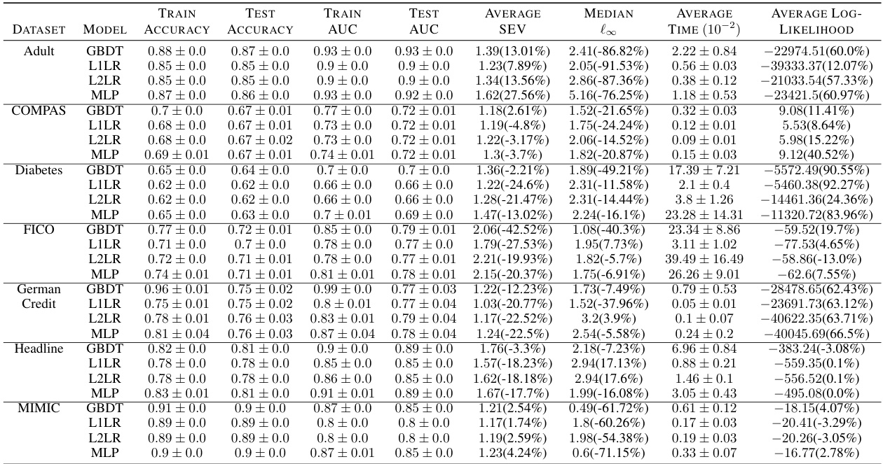
🔼 This table shows an example of how different SEV methods (SEV¹, SEV®, SEVF, SEVT) produce different explanations for the same query point in the FICO dataset. It highlights the impact of different reference point selection strategies on the sparsity and closeness of the explanations. SEV¹ uses a single global reference, while SEV®, SEVF, and SEVT use cluster centers, flexible references, and tree-based methods, respectively, to identify closer and potentially more realistic references. The table illustrates the feature values that changed in each explanation, demonstrating the varying degrees of sparsity achieved by different methods.
read the caption
Table 1: An example for a query in the FICO Dataset with different kinds of explanations, SEV¹ represents the SEV calculation with one single reference using population mean, SEV® represents the cluster-based SEV, SEVF represents the flexible-based SEV. SEVT represents the tree-based SEV The columns are four features.

🔼 This table shows an example of how different SEV methods (SEV¹, SEV©, SEVF, SEVT) produce explanations for a single query in the FICO dataset. SEV¹ uses a single reference point (population mean), while SEV©, SEVF, and SEVT use different reference points and strategies to generate explanations. The table highlights the different feature values that are changed in each explanation to illustrate the differences in sparsity and the approaches of each method.
read the caption
Table 1: An example for a query in the FICO Dataset with different kinds of explanations, SEV¹ represents the SEV calculation with one single reference using population mean, SEV® represents the cluster-based SEV, SEVF represents the flexible-based SEV. SEVT represents the tree-based SEV The columns are four features.

🔼 This table demonstrates the various SEV calculation methods on a single query from the FICO dataset. It compares four different approaches: SEV (using a single reference point as the population mean), cluster-based SEV (using multiple reference points from clusters), flexible-based SEV (allowing for slight adjustments to the reference point), and tree-based SEV (using reference points from decision tree leaves). Each row shows the results for a specific SEV method, highlighting which features were changed in the explanation and the resulting SEV value. This showcases the impact of reference point selection on explanation sparsity.
read the caption
Table 1: An example for a query in the FICO Dataset with different kinds of explanations, SEV¹ represents the SEV calculation with one single reference using population mean, SEV© represents the cluster-based SEV, SEVF represents the flexible-based SEV. SEVT represents the tree-based SEV The columns are four features.
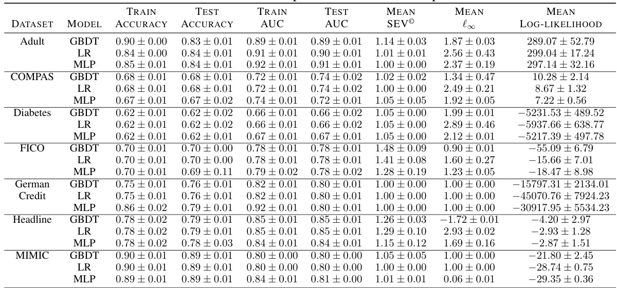
🔼 This table shows an example of how different methods for calculating Sparse Explanation Value (SEV) produce different explanations for a single query in the FICO dataset. It compares four approaches: SEV (using a single reference point), cluster-based SEV (using multiple cluster centers as references), flexible-based SEV (allowing slight adjustments to the reference point), and tree-based SEV (using leaf nodes as references). Each row shows the features that were changed to generate an explanation, along with the resulting SEV for each method.
read the caption
Table 1: An example for a query in the FICO Dataset with different kinds of explanations, SEV¹ represents the SEV calculation with one single reference using population mean, SEV® represents the cluster-based SEV, SEVF represents the flexible-based SEV. SEVT represents the tree-based SEV The columns are four features.

🔼 This table demonstrates the different explanations generated by four different SEV methods for a single query in the FICO dataset. It shows how the choice of reference point and method affects the sparsity of the explanation (number of features changed) and the values of the features that were changed. SEV¹ uses a single reference point (the population mean), while SEV®, SEVF, and SEVT use different methods for selecting reference points and/or allowing flexibility in their positions to achieve more meaningful and sparse explanations.
read the caption
Table 1: An example for a query in the FICO Dataset with different kinds of explanations, SEV¹ represents the SEV calculation with one single reference using population mean, SEV® represents the cluster-based SEV, SEVF represents the flexible-based SEV. SEVT represents the tree-based SEV The columns are four features.

🔼 This table shows an example of how different methods for calculating Sparse Explanation Values (SEV) produce different explanations for the same query point in the FICO dataset. It compares four different SEV approaches: the standard SEV using a single population mean reference (SEV¹), cluster-based SEV (SEV®), flexible-based SEV (SEVF), and tree-based SEV (SEVT). Each row shows the feature values of the query and the modified feature values resulting from each method, along with the calculated SEV for that explanation. The table demonstrates how these different SEV methods can yield explanations with varying levels of sparsity and meaningfulness.
read the caption
Table 1: An example for a query in the FICO Dataset with different kinds of explanations, SEV¹ represents the SEV calculation with one single reference using population mean, SEV® represents the cluster-based SEV, SEVF represents the flexible-based SEV. SEVT represents the tree-based SEV The columns are four features.

🔼 This table demonstrates the different kinds of sparse explanation methods proposed in the paper. Each row represents a query point and its corresponding explanations using different methods. It highlights the differences in terms of the number of features changed and the values of those features, demonstrating how the proposed methods improve sparsity and credibility.
read the caption
Table 1: An example for a query in the FICO Dataset with different kinds of explanations, SEV¹ represents the SEV calculation with one single reference using population mean, SEV© represents the cluster-based SEV, SEVF represents the flexible-based SEV. SEVT represents the tree-based SEV The columns are four features.

🔼 This table shows an example of how different SEV methods produce different explanations for the same query point in the FICO dataset. It compares four methods: SEV (using a single reference point), cluster-based SEV, flexible-based SEV, and tree-based SEV. Each method results in a different set of features that need to be changed to flip the prediction, and each provides a different level of sparsity (number of features changed). The table helps to illustrate the trade-offs and benefits of the different approaches.
read the caption
Table 1: An example for a query in the FICO Dataset with different kinds of explanations, SEV¹ represents the SEV calculation with one single reference using population mean, SEV® represents the cluster-based SEV, SEVF represents the flexible-based SEV. SEVT represents the tree-based SEV The columns are four features.
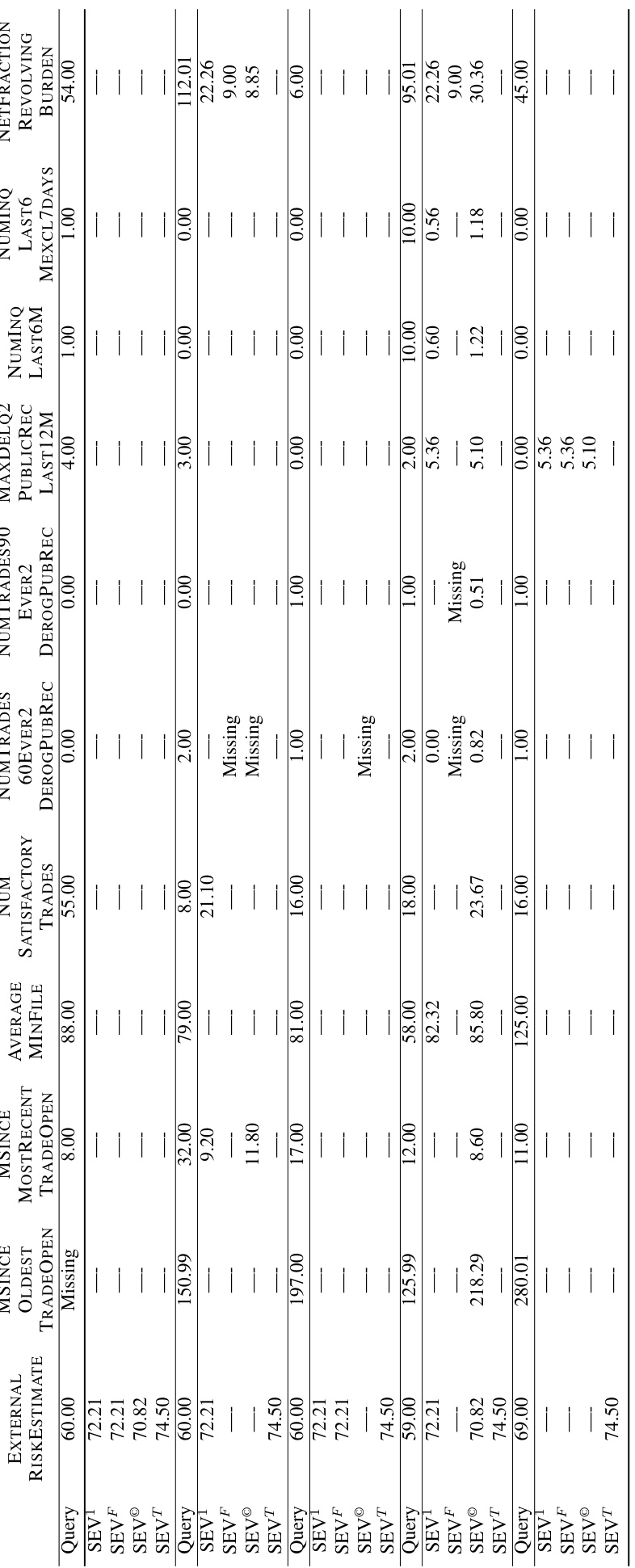
🔼 This table compares four different methods for calculating Sparse Explanation Values (SEV) on a single query from the FICO dataset. SEV¹ uses a single reference point (the population mean). SEV® uses multiple reference points (cluster centers). SEVF allows for flexible reference points, and SEVT is a tree-based variant. The table shows the changes made to four features to obtain a counterfactual explanation for each method, highlighting the different levels of sparsity and closeness achieved.
read the caption
Table 1: An example for a query in the FICO Dataset with different kinds of explanations, SEV¹ represents the SEV calculation with one single reference using population mean, SEV® represents the cluster-based SEV, SEVF represents the flexible-based SEV. SEVT represents the tree-based SEV The columns are four features.
Full paper#
