TL;DR#
Molecular machine learning faces challenges due to the computational costs of training large models on massive datasets. Existing data pruning methods, designed for training from scratch, are often ineffective when used with pre-trained models in the transfer learning paradigm. This incompatibility is largely due to the distribution shift between pre-training and downstream data, common in molecular tasks. This makes efficient training on molecular data challenging, and existing data pruning methods unsuitable for this transfer learning context.
To address this, the paper introduces MolPeg, a novel molecular data pruning framework for enhanced generalization. MolPeg employs a source-free approach, working with pre-trained models, and introduces a unique scoring function based on loss discrepancies between two models (an online model and a reference model with different update paces) to evaluate sample informativeness. MolPeg consistently outperforms existing methods and achieves superior generalization, surpassing full-dataset performance by pruning up to 60-70% of the data in some datasets. This showcases the potential of MolPeg to improve both training efficiency and model generalization, particularly when pre-trained models are used.
Key Takeaways#
Why does it matter?#
This paper is crucial for researchers in molecular machine learning because it introduces a novel, efficient data pruning method. Its success in improving both efficiency and generalization in transfer learning settings significantly impacts the field, opening doors for further research on data-efficient model training and improving the performance of foundation models in molecular tasks. This work directly addresses the computational cost challenges associated with large molecular datasets, which is a major bottleneck in current research.
Visual Insights#

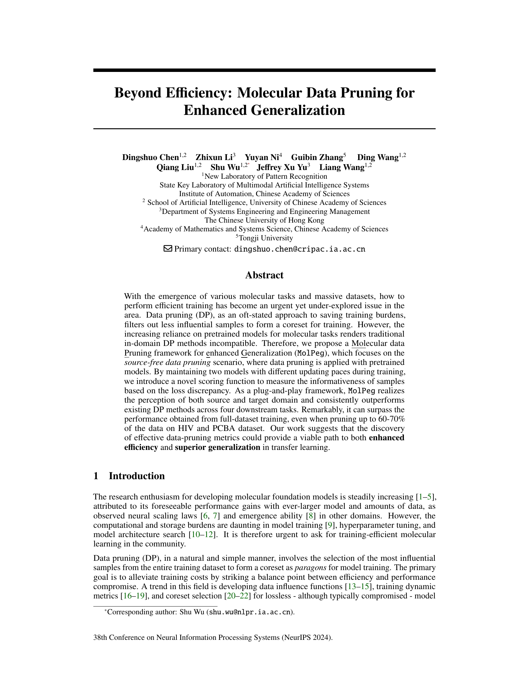
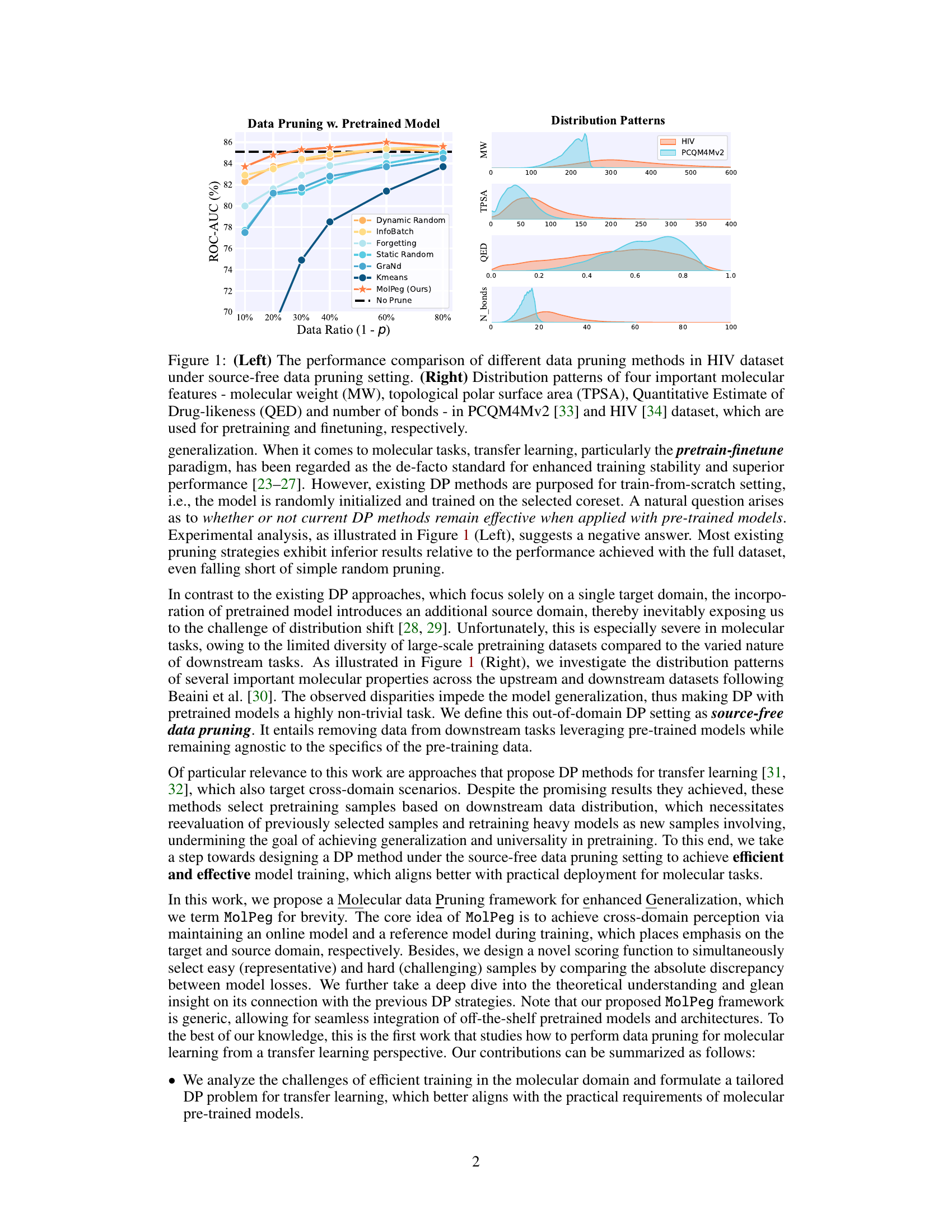
🔼 The figure compares various data pruning methods’ performance on the HIV dataset in a source-free setting (left panel). It also shows the distribution patterns of four key molecular features (MW, TPSA, QED, and number of bonds) in both the PCQM4Mv2 (pretraining) and HIV (finetuning) datasets (right panel), highlighting the distribution shift between the source and target domains. This visualization helps explain the challenges of applying traditional data pruning methods to transfer learning scenarios in molecular tasks.
read the caption
Figure 1: (Left) The performance comparison of different data pruning methods in HIV dataset under source-free data pruning setting. (Right) Distribution patterns of four important molecular features - molecular weight (MW), topological polar surface area (TPSA), Quantitative Estimate of Drug-likeness (QED) and number of bonds - in PCQM4Mv2 [33] and HIV [34] dataset, which are used for pretraining and finetuning, respectively.
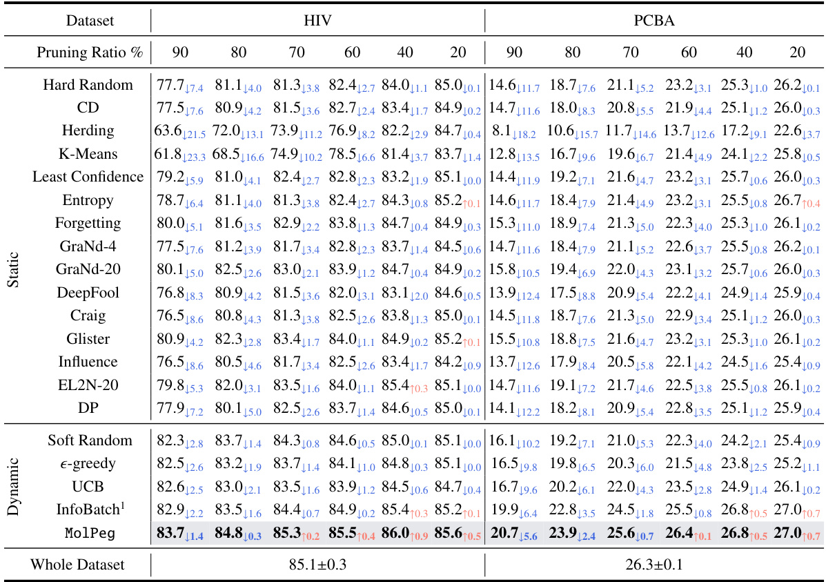
🔼 This table presents a comparison of the performance of various data pruning methods (including MolPeg) on the HIV and PCBA datasets. The performance metrics used are ROC-AUC and Average Precision. The table highlights the best-performing method for each pruning ratio and shows the performance difference compared to using the whole dataset. This allows for easy comparison of the effectiveness and efficiency of different pruning techniques.
read the caption
Table 1: The performance comparison to state-of-the-art methods on HIV and PCBA in terms of ROC-AUC (%, ↑) and Average Precision (%, ↑). We highlight the best-performing results in boldface. The performance difference with whole dataset training is highlighted with blue and orange, respectively.
In-depth insights#
MolPeg Framework#
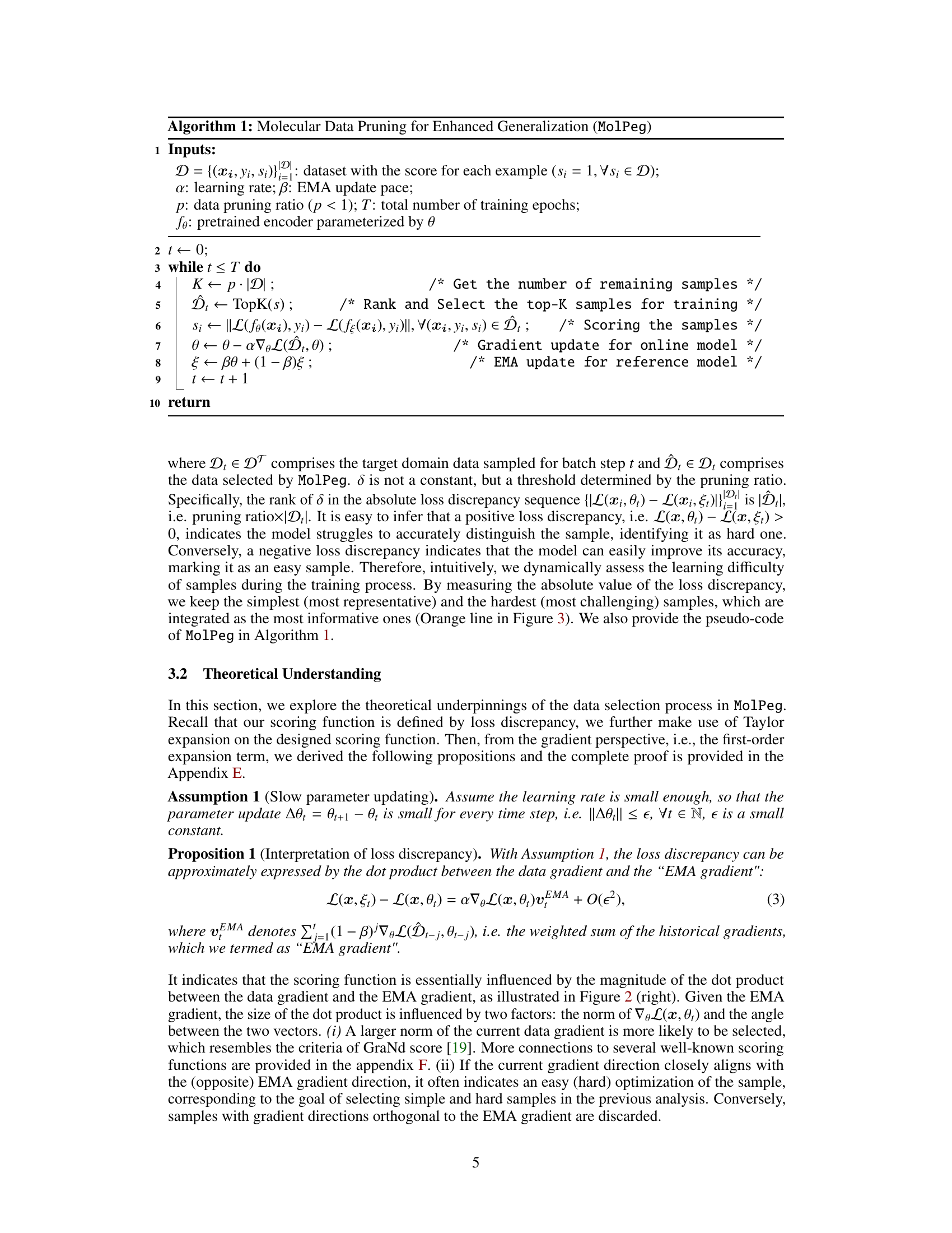
The MolPeg framework, designed for enhanced generalization in molecular data pruning, cleverly addresses the challenge of source-free pruning. It employs two models: an online model focusing on the target domain and a reference model leveraging pre-trained knowledge from the source domain. A novel scoring function, based on the loss discrepancy between these models, effectively measures the informativeness of samples. This dual-model approach enables MolPeg to perceive both source and target domains without needing the source data. Furthermore, MolPeg’s selection process incorporates both easy and hard samples, striking a balance between fast adaptation and robust generalization. The framework’s plug-and-play nature and consistent outperformance highlight its potential for efficient and effective transfer learning in molecular tasks.
Source-Free Pruning#
Source-free pruning presents a novel approach to data pruning in transfer learning settings, particularly relevant for resource-intensive domains like molecular modeling. Traditional data pruning methods often rely on access to the source data, which is unavailable in this context. Source-free pruning addresses this limitation by leveraging pre-trained models to guide the selection of informative samples from the target domain alone. This eliminates the need for source data and its associated limitations. The key challenge in source-free pruning is developing effective metrics to assess the informativeness of samples without explicit knowledge of the source distribution. The success of this approach hinges on accurately capturing the knowledge transfer from the pre-trained model. This often involves designing sophisticated scoring functions that capture the model’s behavior in the target domain. Furthermore, careful consideration of downstream task specifics is critical, as transfer learning performance may be sensitive to the characteristics of the target dataset and the pre-trained model’s generalization capabilities. While promising, further research is needed to fully understand the theoretical underpinnings of effective source-free pruning metrics and their robustness across diverse transfer learning scenarios.
Cross-Domain Scoring#
Cross-domain scoring, in the context of a research paper dealing with molecular data pruning and transfer learning, likely refers to a method for evaluating the importance of data samples by considering their relevance to both a source and a target domain. A core challenge in transfer learning is the distribution shift between these domains. Effective cross-domain scoring would need to capture this distribution shift, weighing samples not just by their individual informativeness within the target domain but also by how much information they provide about the relationship between source and target distributions. This might involve comparing model outputs or loss functions on pre-trained models (source domain) and fine-tuned models (target domain) for each sample. A good cross-domain scoring metric would therefore need to be robust to domain discrepancies, and ideally, provide a principled way of combining information from the two domains to prioritize samples that are both informative and representative of the target task, while also helping to bridge the gap between the source and target distributions. A good metric should also be computationally efficient enough for large-scale molecular datasets.
Generalization Gains#
Analyzing the concept of “Generalization Gains” in a research paper requires understanding how well a model trained on a specific dataset performs on unseen data. High generalization suggests the model has learned underlying patterns, not just memorized the training set. A key aspect is the evaluation metrics used; accuracy alone might be insufficient, and other measures like precision, recall, and F1-score offer more comprehensive insights. Factors influencing generalization include dataset size and diversity, model architecture, and training techniques (e.g., regularization). A well-generalizing model exhibits robustness against noisy data and variations in input distribution. The paper likely investigates how these factors interact, perhaps comparing different training approaches or model designs, quantifying the extent of generalization gains achieved and explaining why certain methods outperform others. The discussion would ideally cover the trade-off between efficiency and generalization; more efficient training methods might sacrifice some generalization, while highly generalizable models can demand greater computational resources.
Future Directions#
Future research could explore extending MolPeg’s applicability beyond molecular datasets to other domains like natural language processing or computer vision, where transfer learning is prevalent. Investigating more sophisticated methods for measuring sample informativeness, potentially incorporating second-order gradient information or other advanced metrics, could lead to improved pruning accuracy. Furthermore, adaptive pruning strategies that dynamically adjust pruning ratios based on the model’s performance would enhance efficiency and robustness. A deeper theoretical analysis exploring the connections between MolPeg and other coreset selection methods is warranted to better understand its strengths and limitations. Finally, applying MolPeg to larger-scale datasets and more complex molecular tasks will further validate its effectiveness and scalability in real-world applications.
More visual insights#
More on figures

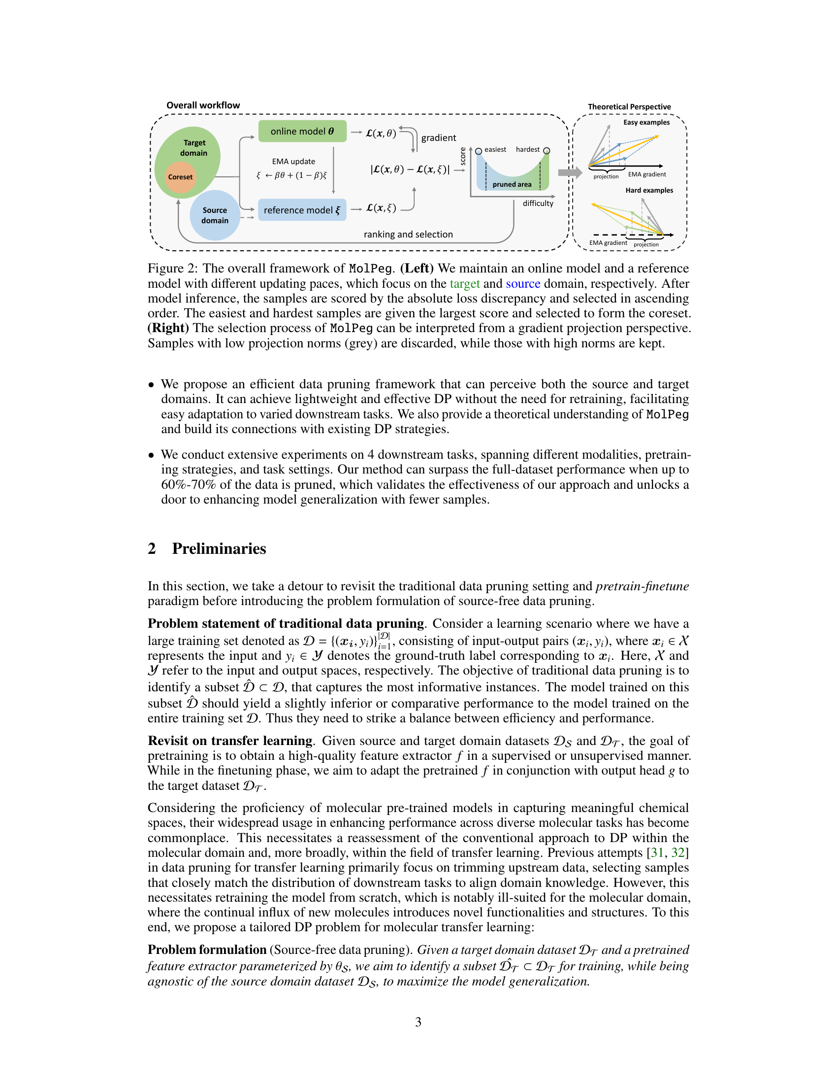
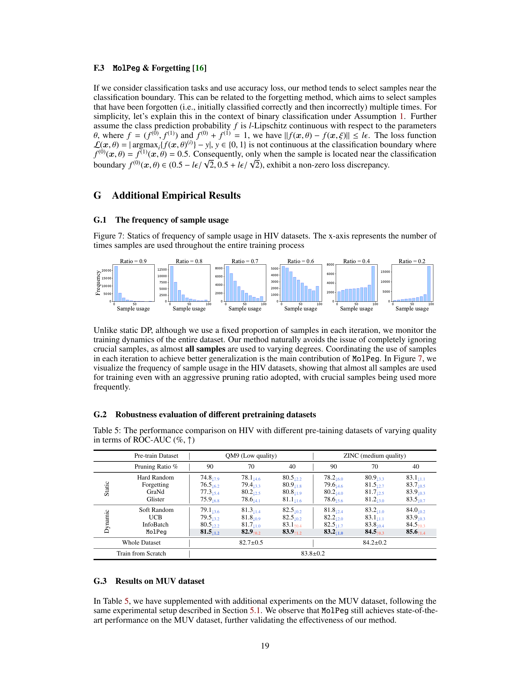
🔼 This figure illustrates the MolPeg framework. The left panel shows the overall workflow, highlighting the use of an online model and a reference model with different update speeds to process samples from the target and source domains. Samples are scored based on the absolute loss discrepancy between the two models and ranked. The easiest and hardest samples are selected to form the coreset. The right panel provides a theoretical perspective, illustrating how the selection process can be viewed as a gradient projection. Samples with low projection norms are discarded, while those with high norms are retained.
read the caption
Figure 2: The overall framework of MolPeg. (Left) We maintain an online model and a reference model with different updating paces, which focus on the target and source domain, respectively. After model inference, the samples are scored by the absolute loss discrepancy and selected in ascending order. The easiest and hardest samples are given the largest score and selected to form the coreset. (Right) The selection process of MolPeg can be interpreted from a gradient projection perspective.
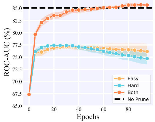
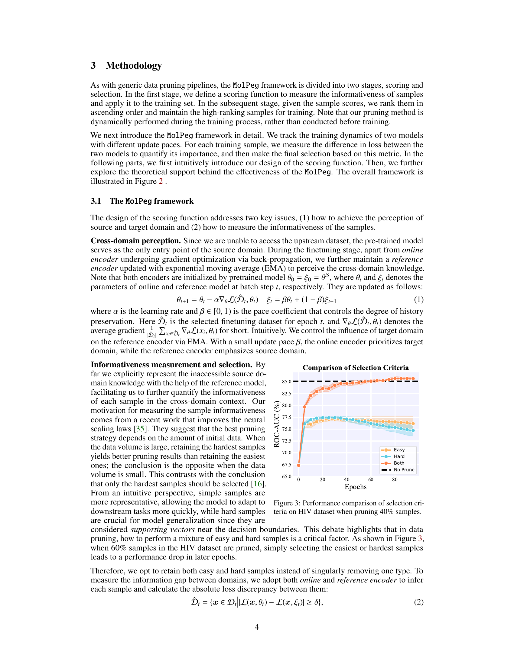
🔼 This figure compares the performance of three different sample selection strategies (selecting only easy samples, only hard samples, or both) within the MolPeg framework. The x-axis represents the training epoch, and the y-axis shows the ROC-AUC score. The results demonstrate that selecting both easy and hard samples leads to the best performance, outperforming strategies that only select easy or hard samples. The black dashed line represents the ROC-AUC achieved by training on the full dataset (no pruning). The shaded area around each line represents the standard deviation across multiple runs.
read the caption
Figure 3: Performance comparison of selection criteria on HIV dataset when pruning 40% samples.
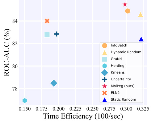
🔼 The figure shows a comparison of different data pruning methods’ performance on an HIV dataset, considering a scenario where data pruning is applied using pre-trained models. The left panel illustrates the performance comparison of various methods at different pruning ratios. The right panel displays the distribution patterns of key molecular features in the PCQM4Mv2 (pretraining) and HIV (finetuning) datasets to highlight the distribution shift challenge.
read the caption
Figure 1: (Left) The performance comparison of different data pruning methods in HIV dataset under source-free data pruning setting. (Right) Distribution patterns of four important molecular features - molecular weight (MW), topological polar surface area (TPSA), Quantitative Estimate of Drug-likeness (QED) and number of bonds - in PCQM4Mv2 [33] and HIV [34] dataset, which are used for pretraining and finetuning, respectively.

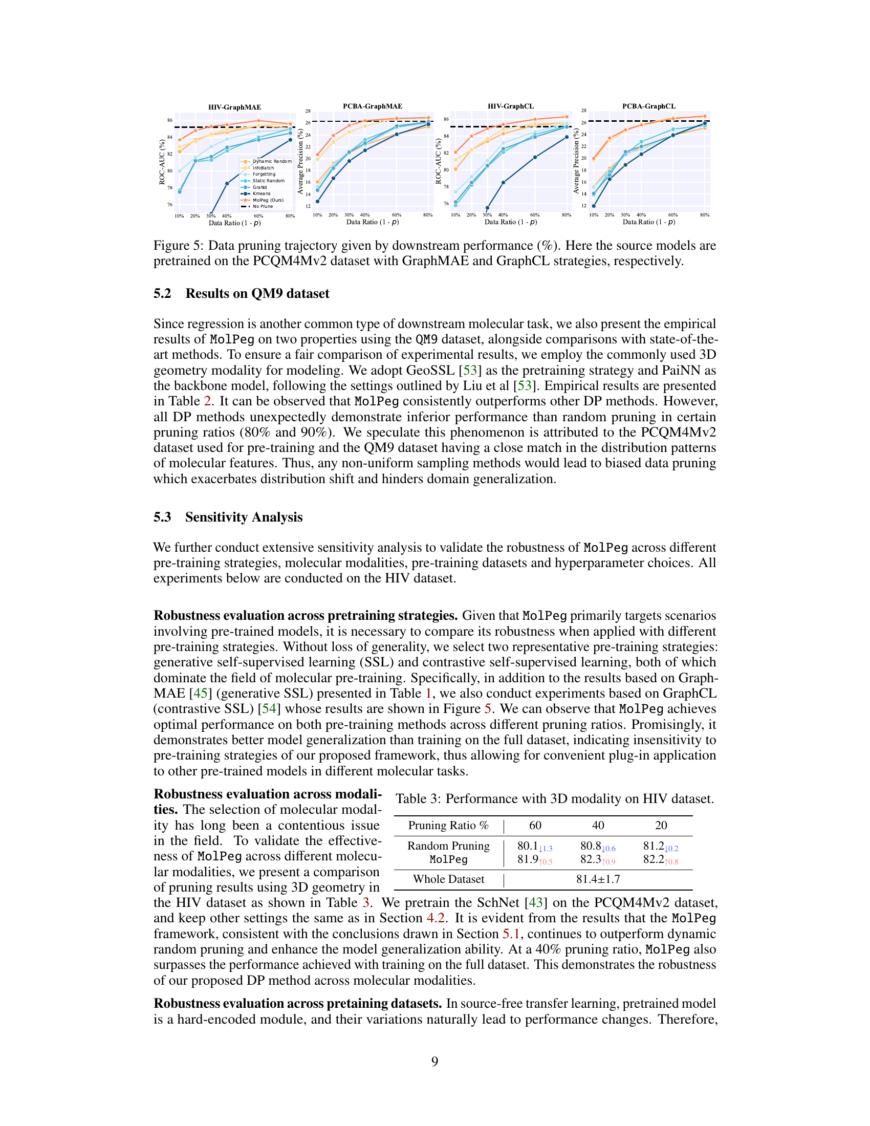
🔼 This figure compares the performance of different data pruning methods on two datasets (HIV and PCBA) using two different pre-training strategies (GraphMAE and GraphCL). The x-axis represents the percentage of data retained after pruning (Data Ratio (1-p)), ranging from 10% to 80%. The y-axis shows the performance measured by ROC-AUC (%) for HIV and Average Precision (%) for PCBA. The lines represent different data pruning methods, including MolPeg (the proposed method) and several baselines. The horizontal dashed lines indicate the performance achieved without any pruning (No Prune). The figure demonstrates that MolPeg consistently outperforms other methods across different pruning ratios and pre-training strategies.
read the caption
Figure 5: Data pruning trajectory given by downstream performance (%). Here the source models are pretrained on the PCQM4Mv2 dataset with GraphMAE and GraphCL strategies, respectively.

🔼 This figure shows the performance of MolPeg model on the HIV dataset with different values of hyperparameter β. The x-axis represents the pruning ratio (0.1, 0.4, and 0.8), and the y-axis represents the ROC-AUC. Different colors represent different values of β (0.001, 0.01, 0.1, 0.5, and 0.9). Error bars indicate the standard deviation. The results suggest that the performance of MolPeg model is relatively insensitive to the choice of β, with β=0.5 achieving a good balance between performance and stability.
read the caption
Figure 6: Performance bar chart of different choices of hyper-parameter β on HIV dataset. The error bar is measured in standard deviation and plotted in grey color.

🔼 The figure shows the comparison of different data pruning methods’ performance on the HIV dataset under a source-free setting (left). It also illustrates the distribution patterns of key molecular features (MW, TPSA, QED, number of bonds) in the PCQM4Mv2 and HIV datasets used for pre-training and fine-tuning, respectively (right). The left panel highlights the performance of MolPeg in comparison to other methods, while the right panel illustrates the distribution differences between the source (pre-training) and target (fine-tuning) datasets, motivating the need for a source-free data pruning method.
read the caption
Figure 1: (Left) The performance comparison of different data pruning methods in HIV dataset under source-free data pruning setting. (Right) Distribution patterns of four important molecular features - molecular weight (MW), topological polar surface area (TPSA), Quantitative Estimate of Drug-likeness (QED) and number of bonds - in PCQM4Mv2 [33] and HIV [34] dataset, which are used for pretraining and finetuning, respectively.
More on tables

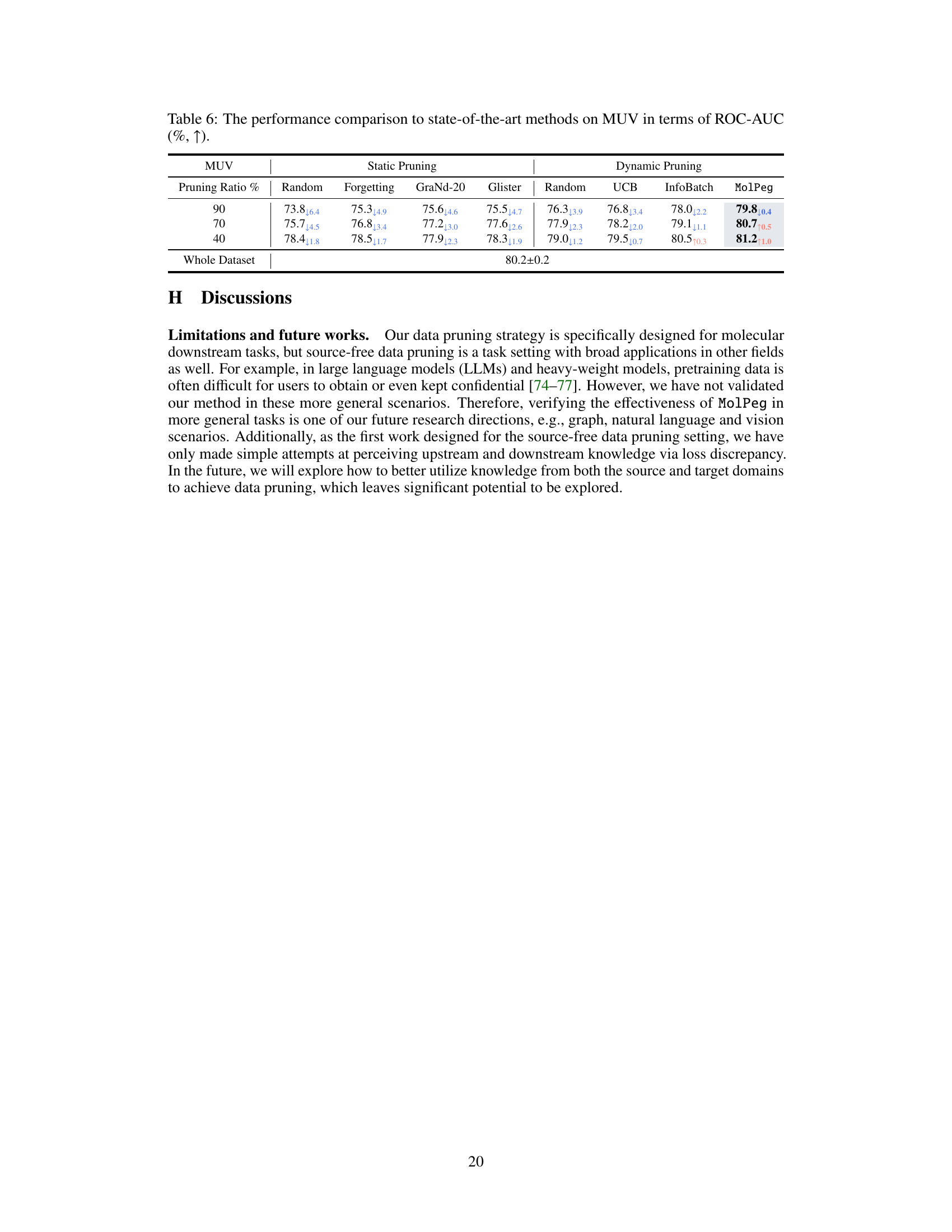
🔼 This table presents a comparison of the performance of MolPeg against other state-of-the-art data pruning methods on the QM9 dataset. The performance metric used is Mean Absolute Error (MAE), with lower values indicating better performance. The table shows results for different pruning ratios (percentage of data removed) and highlights the best and second-best performing methods for each ratio in bold and underlined text, respectively. The results are for two different properties in QM9, QM9-U0 and QM9-Zpve.
read the caption
Table 2: The performance comparison to state-of-the-art methods on QM9 dataset in terms of MAE (↓). We highlight the best- and the second-performing results in boldface and underlined, respectively.

🔼 This table presents the performance comparison of different data pruning methods on the HIV dataset using the 3D modality. It shows the ROC-AUC scores for various pruning ratios (60%, 40%, 20%) for Random Pruning and MolPeg, and also includes the performance of training with the whole dataset. The results highlight the effectiveness of MolPeg in achieving superior performance compared to random pruning, even surpassing the full dataset performance at certain pruning ratios.
read the caption
Table 3: Performance with 3D modality on HIV dataset.

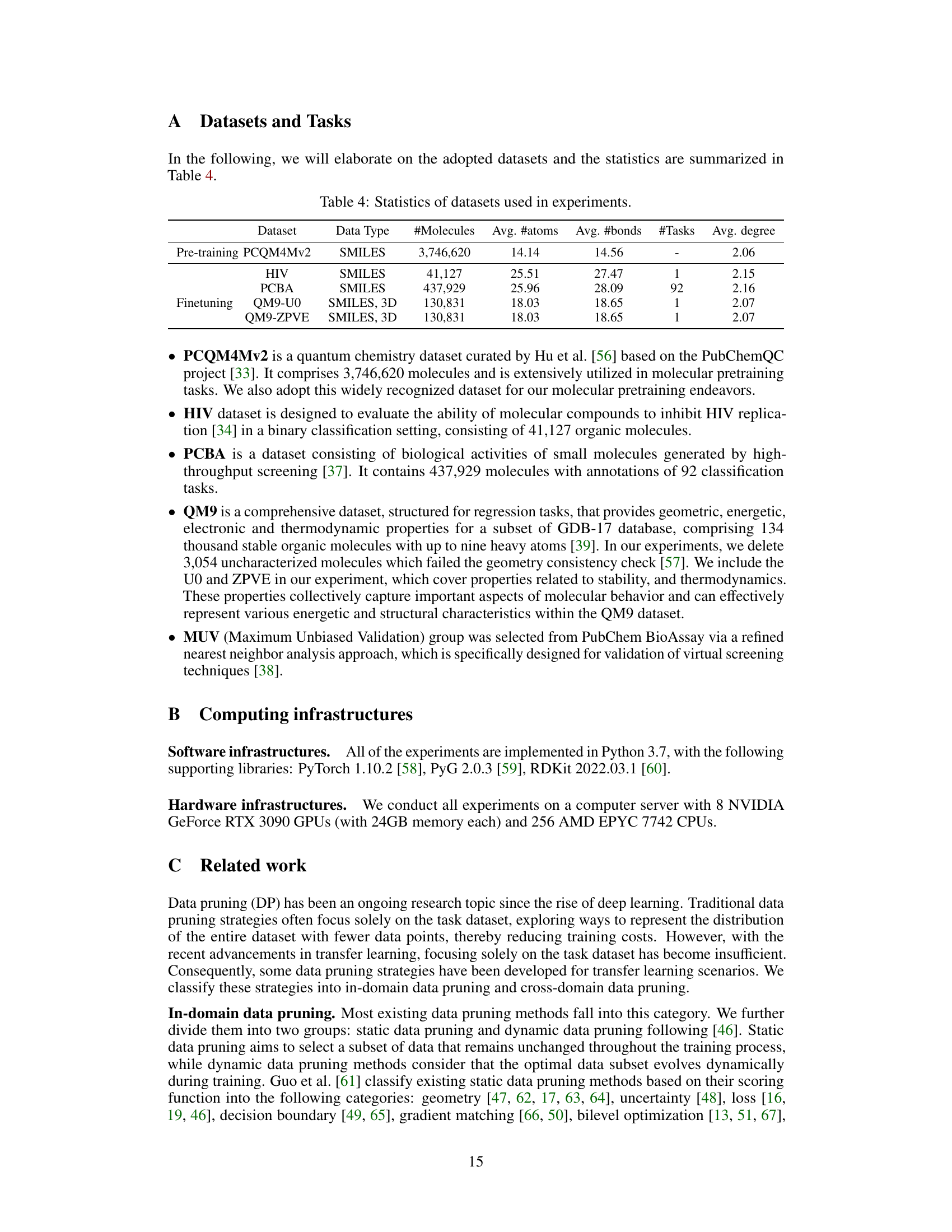
🔼 This table presents a summary of the datasets used in the experiments described in the paper. It shows the dataset name, data type (SMILES or SMILES, 3D), the number of molecules, the average number of atoms and bonds per molecule, the number of tasks (for multi-task datasets), and the average degree of the molecular graphs. The datasets are categorized into pre-training datasets (used to train the initial model) and finetuning datasets (used to adapt the pre-trained model to specific tasks).
read the caption
Table 4: Statistics of datasets used in experiments.

🔼 This table presents the results of the robustness evaluation across pretaining datasets. It compares the performance of various data pruning methods (Hard Random, Forgetting, GraNd, Glister, Soft Random, UCB, InfoBatch, MolPeg) on the HIV dataset, using two pretrained models of varying quality, obtained from the ZINC15 and QM9 datasets. The results are shown for three different pruning ratios (90%, 70%, 40%). The table also includes the performance of training on the full dataset and training from scratch for comparison.
read the caption
Table 5: The performance comparison on HIV with different pre-taining datasets of varying quality in terms of ROC-AUC (%, ↑)

🔼 This table presents the performance comparison of different data pruning methods on the MUV dataset in terms of ROC-AUC. It shows the results for both static and dynamic pruning methods at different pruning ratios (90%, 70%, and 40%). The methods compared include random pruning, forgetting, GraNd-20, Glister, UCB, InfoBatch, and MolPeg. The table highlights the best-performing results, allowing for a direct comparison of the effectiveness of each method at different data reduction levels.
read the caption
Table 6: The performance comparison to state-of-the-art methods on MUV in terms of ROC-AUC (%, ↑).
Full paper#
