TL;DR#
Estimating unknown functions from expensive evaluations is crucial in many fields. Existing methods like Bayesian Optimization focus on extreme values, while experimental design aims for global estimation. Both approaches have limitations; Bayesian Optimization neglects the broader function landscape, while experimental design is computationally expensive. Level set estimation offers a compromise, but requires threshold selection, which is problematic without prior knowledge.
This paper introduces ‘active set ordering,’ a novel framework that efficiently estimates subsets of inputs based on pairwise orderings determined from expensive evaluations. It proposes the ‘Mean Prediction’ algorithm and provides theoretical analysis based on regret. The framework is demonstrated on synthetic functions and real datasets, showing improvements compared to other methods. It also connects to Bayesian Optimization as a special case, providing a unified perspective.
Key Takeaways#
Why does it matter?#
This paper is important because it formalizes a new problem, active set ordering, which bridges the gap between global function estimation and Bayesian optimization. It offers a theoretically grounded solution with sublinear regret, providing valuable insights for various applications involving expensive black-box function evaluations, opening avenues for further research in efficient data acquisition strategies and improved algorithm design. The solution also recovers existing algorithms like GP-UCB, providing a unified framework.
Visual Insights#
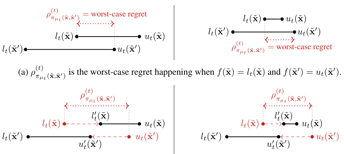
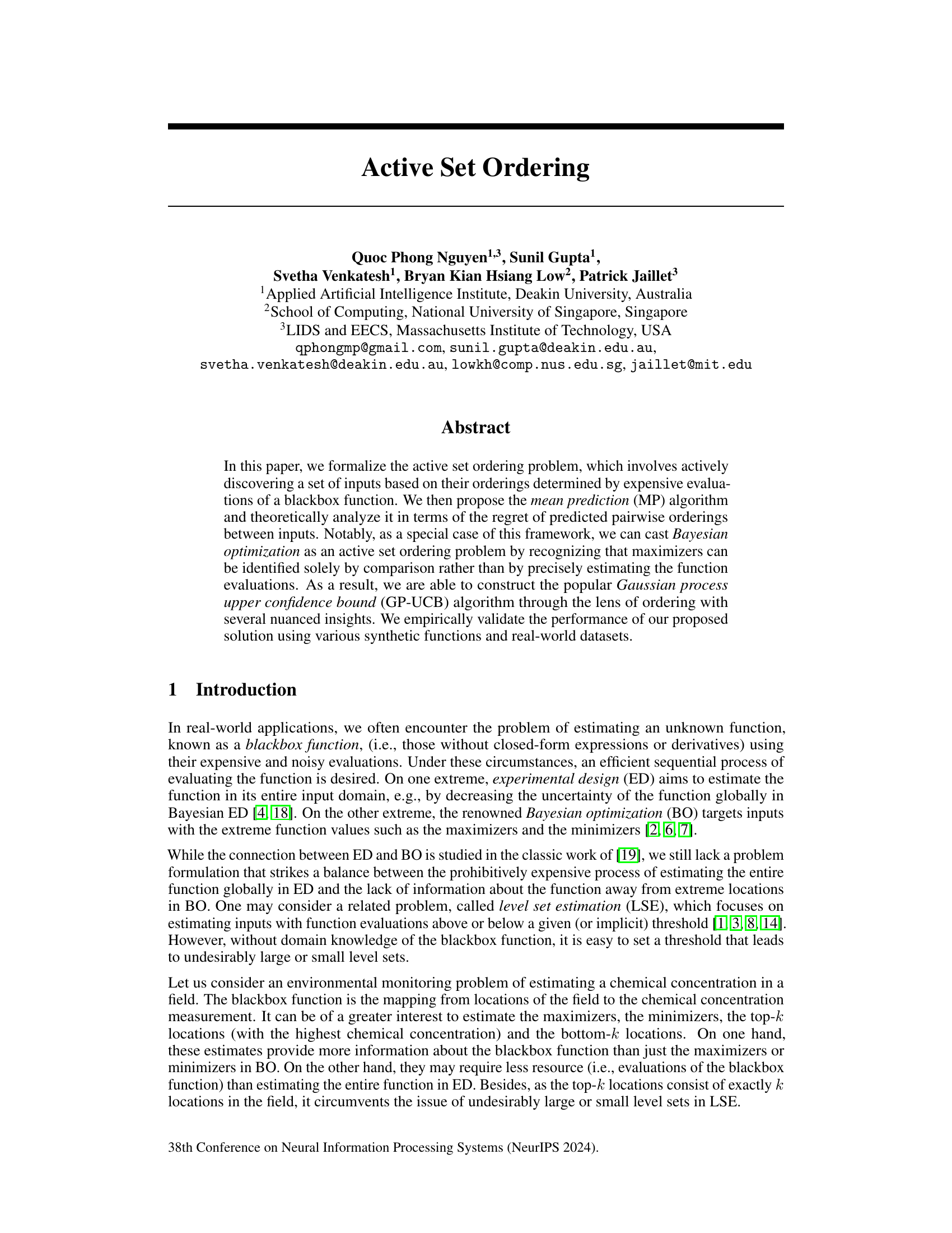
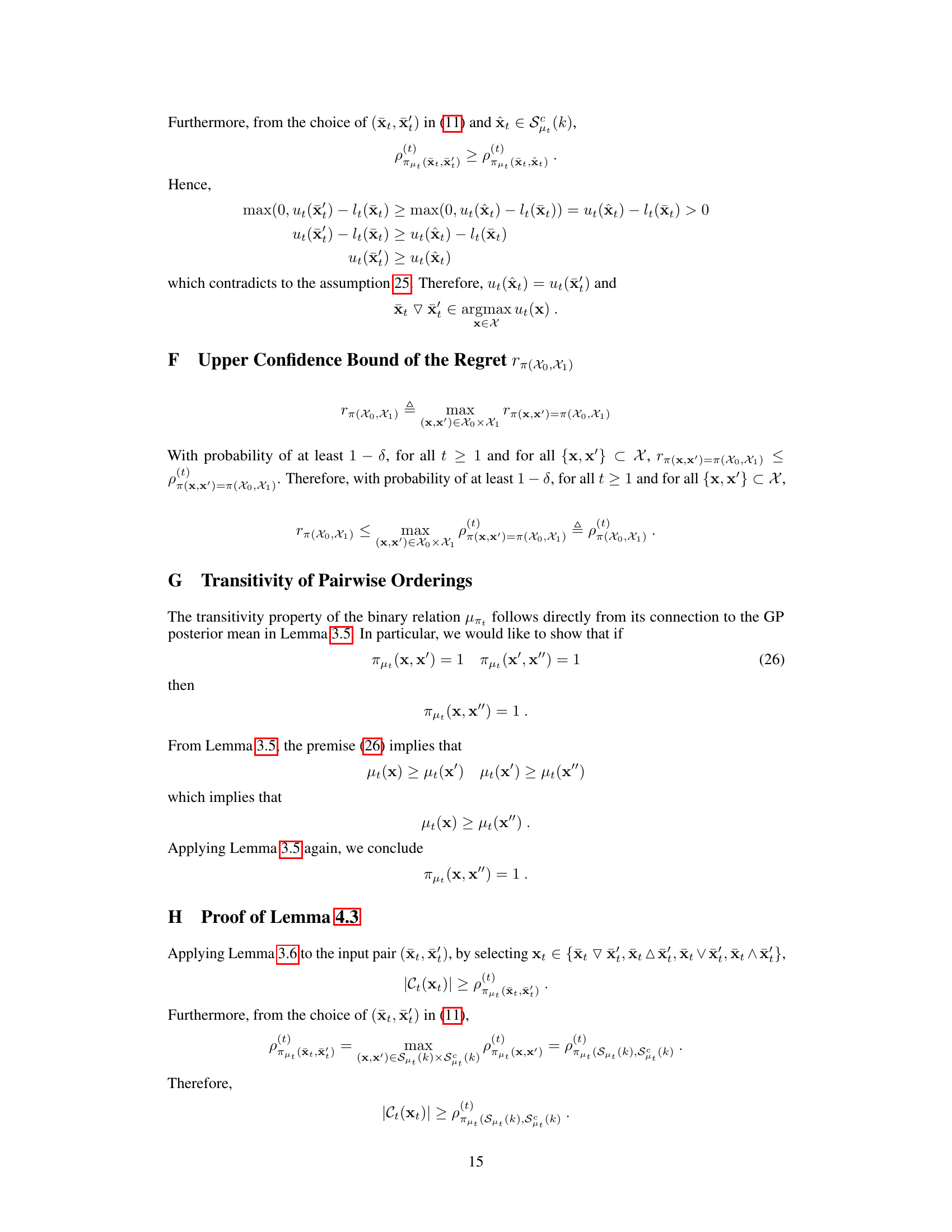
🔼 This figure illustrates two interpretations of the upper bound ρπμε (x,x’) on the regret when the predicted ordering πμε (x, x’) is 1. Panel (a) shows that ρπμε (x,x’) represents the worst-case regret that occurs when the true function values are at the lower confidence bound for x and the upper confidence bound for x’. Panel (b) shows that ρπμε (x,x’) represents the minimum reduction in uncertainty needed to ensure that the predicted ordering is correct with high probability, shown as the sum of the lengths of the two red segments.
read the caption
Figure 1: Interpretations of the upper bound ρπμε (x,x') when πμε (x, x') = 1.
In-depth insights#
Active Set Ordering#
Active set ordering presents a novel approach to efficiently estimate subsets of inputs from a black box function, striking a balance between the exhaustive exploration of Bayesian experimental design and the extreme-value focus of Bayesian optimization. The core idea is to iteratively select inputs based on pairwise comparisons, focusing on the orderings rather than precise function values. This framework allows for the estimation of various sets, such as maximizers, minimizers, and top-k elements, providing more comprehensive information than traditional BO. The proposed algorithm employs Gaussian processes to model the function uncertainty and incorporates a novel regret definition to guide the input selection process. Theoretical analysis provides performance guarantees, and empirical results validate its efficiency on both synthetic functions and real-world datasets. The approach also offers valuable insights into the relationship between active learning, Bayesian optimization, and level set estimation, unifying these concepts under a single framework.
Regret Analysis#
Regret analysis in the context of active learning and black-box function optimization is crucial for evaluating the efficiency of algorithms. It quantifies the difference between the performance of an algorithm and the optimal strategy in hindsight. In this setting, the algorithm sequentially selects inputs for evaluation, aiming to maximize some utility function, such as finding the global maximum or estimating a level set. The cumulative regret measures the total loss accrued due to suboptimal decisions. A key goal in this field is designing algorithms with sublinear regret, indicating that the algorithm’s performance converges towards optimal as the number of queries increases. Different types of regret exist, depending on the precise definition of loss (e.g., pairwise comparison regret or top-k set regret). Theoretical analysis often focuses on deriving upper bounds on the cumulative regret, giving insights into algorithm performance and scalability. Empirical evaluations demonstrate regret bounds, with comparisons made to naive or random strategies. Understanding and minimizing regret is essential for improving the efficiency and effectiveness of active learning methods applied to a broad range of real-world problems where function evaluations are expensive or time-consuming. The design of efficient regret-minimizing strategies is a central research area.
GP-UCB Recovery#
The heading ‘GP-UCB Recovery’ suggests a key finding: the proposed active set ordering method successfully recovers the well-known Gaussian Process Upper Confidence Bound (GP-UCB) algorithm as a special case. This is significant because it establishes a theoretical connection between two seemingly disparate approaches: Bayesian Optimization (BO), which focuses on finding extreme values, and active set ordering, which aims for broader set estimation based on ordering comparisons. The recovery is not merely algorithmic but also theoretical, encompassing both the GP-UCB algorithm itself and its associated regret bound analysis. This unified perspective provides valuable insights into the underlying principles of both methodologies, possibly revealing new optimization strategies and facilitating algorithm design within a more general framework. The ability to derive a well-established algorithm like GP-UCB as a specific instance of the active set ordering approach strengthens the novelty and significance of the proposed method, highlighting its potential as a more comprehensive solution for black-box function optimization.
MP Algorithm#
The MP (Mean Prediction) algorithm, as presented in the research paper, offers a novel approach to the active set ordering problem. Its core innovation lies in framing Bayesian optimization as a special case of active set ordering, enabling a more unified perspective on the problem. The algorithm cleverly uses the posterior mean of a Gaussian Process to predict pairwise orderings of function evaluations, thereby avoiding the need for precise function estimations, which are often computationally expensive. The algorithm’s theoretical foundation is grounded in a novel regret definition, allowing for a rigorous analysis of its performance. This analysis leads to a sampling strategy that guarantees sublinear cumulative regret under certain conditions, thus ensuring efficient exploration of the input space. The MP algorithm is particularly noteworthy for recovering the GP-UCB algorithm as a special case, offering a fresh perspective on the existing methodology and potentially paving the way for improved optimization strategies. Furthermore, the algorithm shows promising empirical performance across several synthetic and real-world datasets.
Future Extensions#
Future research directions stemming from this active set ordering framework are plentiful. Extending the theoretical analysis to handle more complex noise models beyond Gaussian noise is crucial for broader applicability. Investigating alternative acquisition functions to the mean prediction (MP) approach, potentially leveraging ideas from other active learning paradigms, could improve performance. Empirical evaluation on a wider range of high-dimensional real-world datasets is essential to fully assess the robustness and scalability of the proposed method. Furthermore, developing efficient algorithms to handle the computational challenges posed by high dimensionality is a critical next step. Finally, exploring the theoretical connections between active set ordering and other related problems such as level-set estimation and Bayesian optimization in greater depth could uncover further unifying principles and lead to more efficient algorithms.
More visual insights#
More on figures

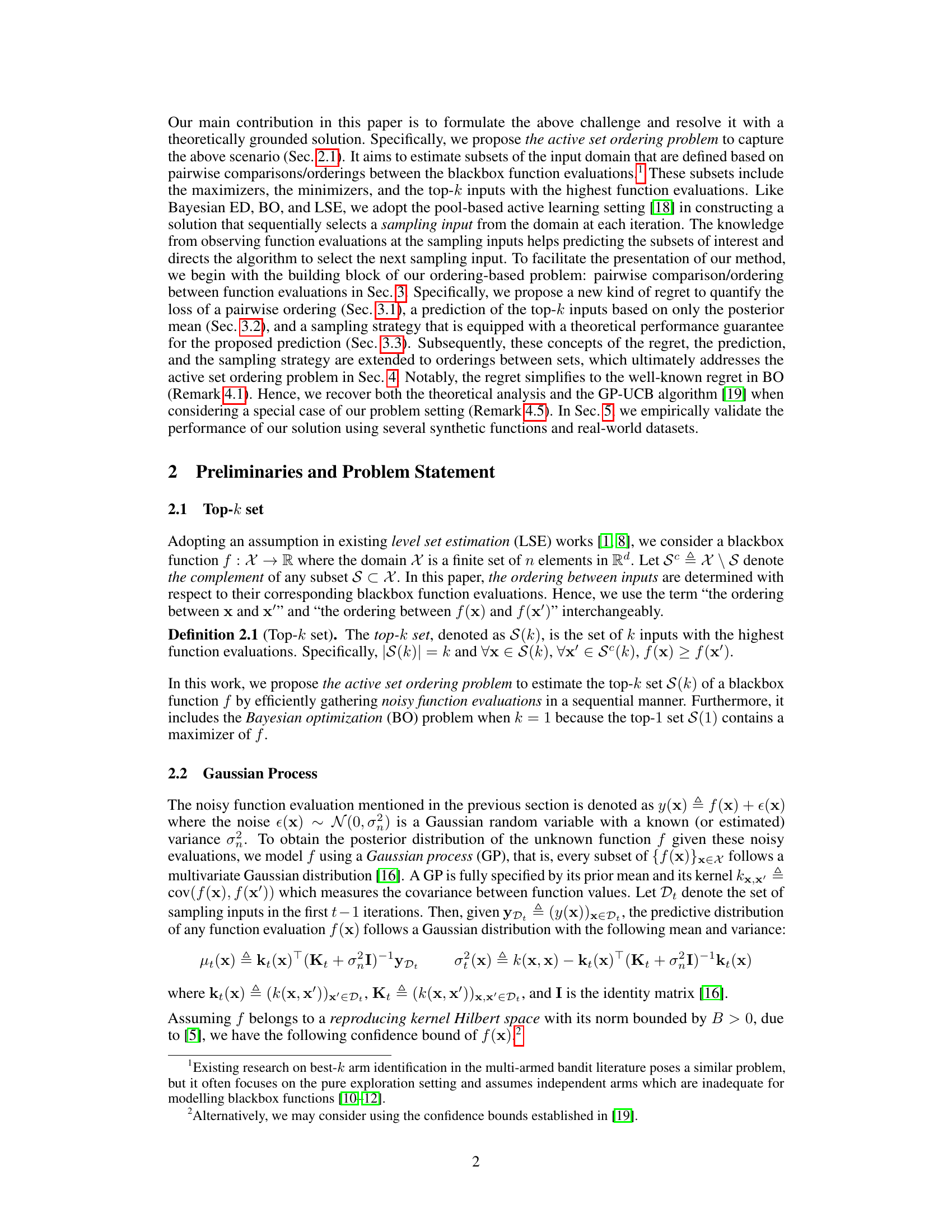
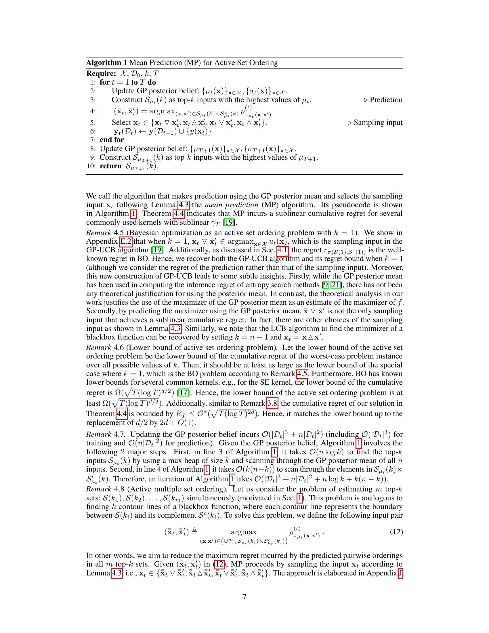
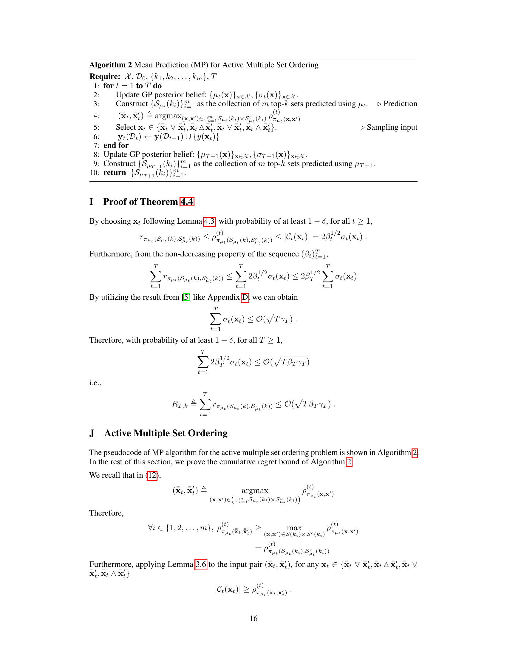
🔼 This figure compares the performance of two algorithms, MP and Var, in estimating the top 20 inputs (S(20)) of a synthetic function. The MP algorithm uses a novel mean prediction approach, while Var is a baseline uncertainty sampling method. The plots show the sampling inputs selected by each algorithm over 40 iterations, along with the GP posterior mean, upper and lower confidence bounds, and the true top 20 inputs. The histograms show the distribution of sampling inputs across the input domain for each algorithm. The figure highlights how the MP algorithm focuses sampling on the boundary region of the top 20 inputs, whereas the Var algorithm samples more uniformly across the input space.
read the caption
Figure 2: Plot of sampling inputs, GP posterior distribution, and the performance of (a) MP and (b) Var in estimating S(20) of a synthetic function. The comparison pair is (xt, x) in (11). The histogram on the horizontal axis shows the frequency of sampling inputs in 40 iterations.

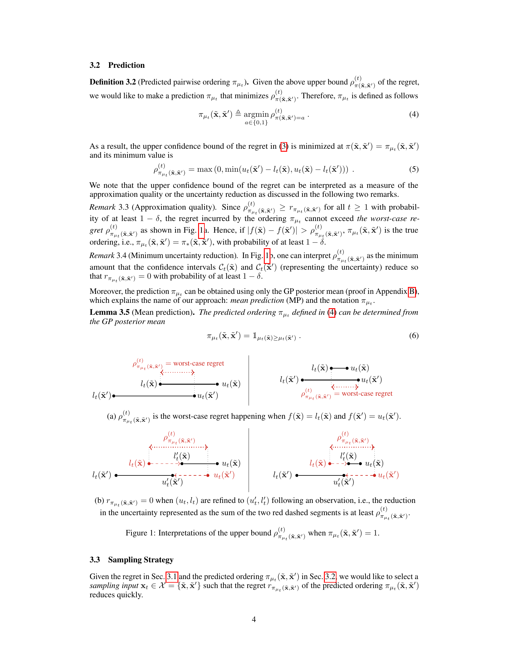
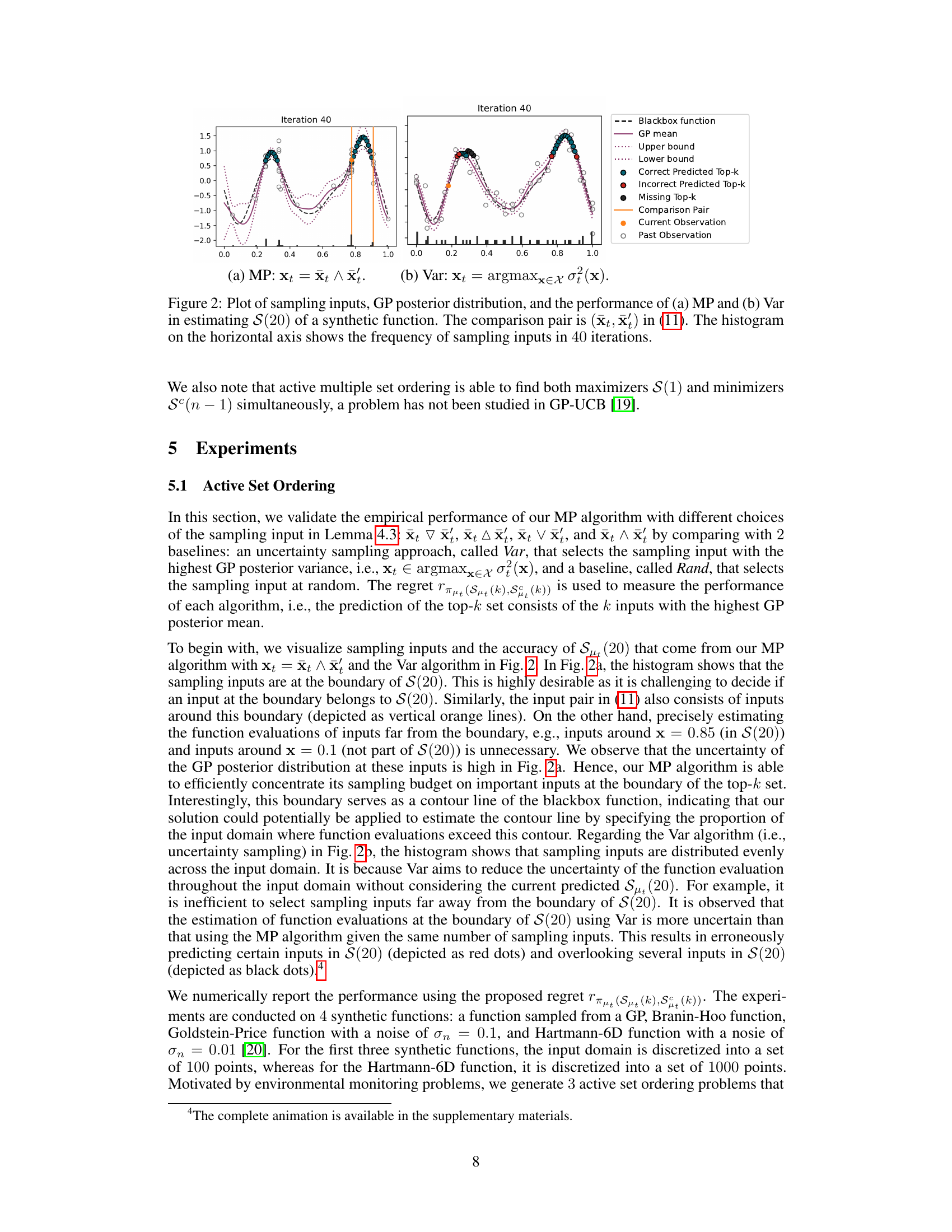
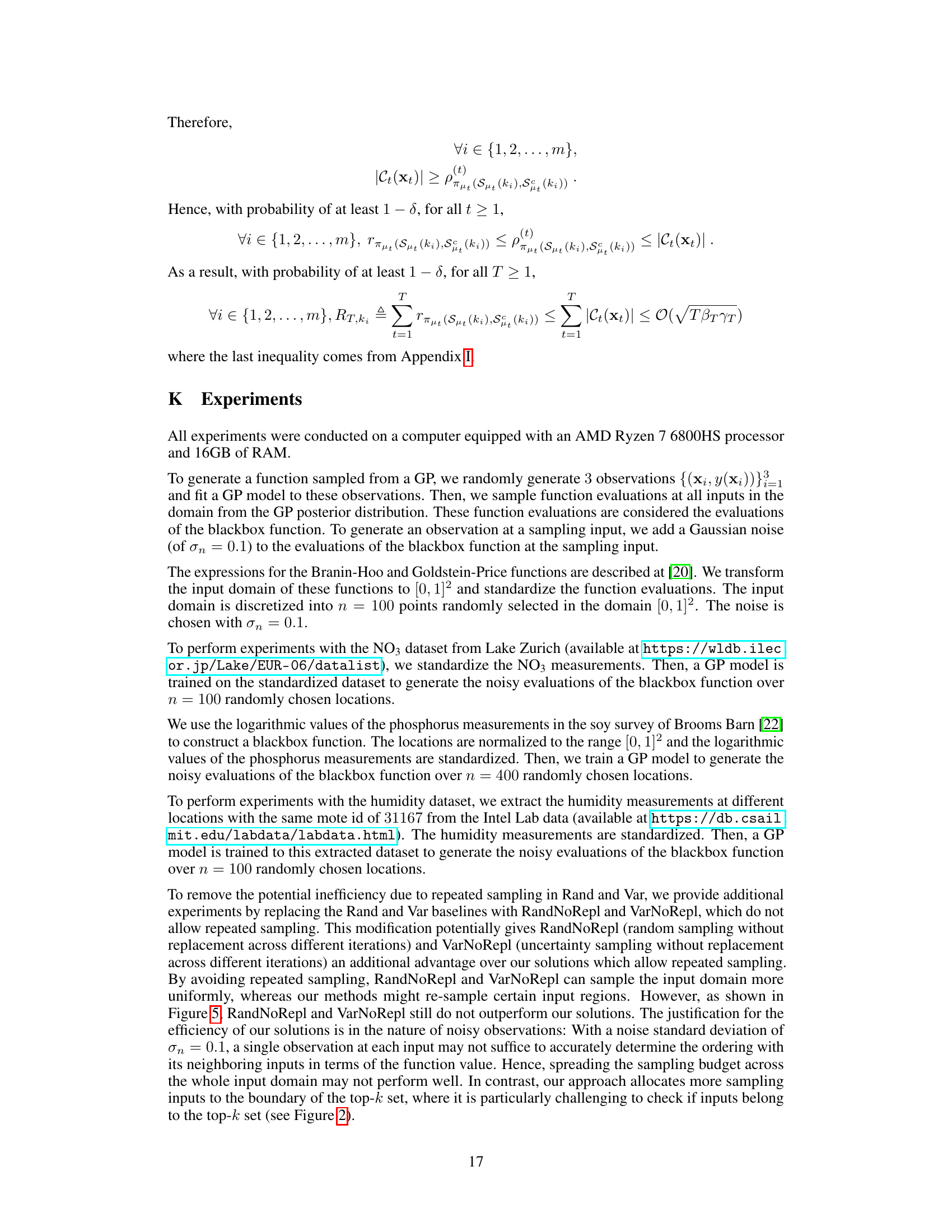
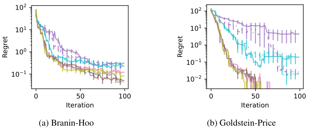
🔼 This figure displays the performance of different algorithms in estimating top-k sets of a blackbox function. The top row (s:a-d) shows results for estimating the top 5 elements (k=5) across four different test functions (GP sample, Branin-Hoo, Goldstein-Price, Hartmann-6D), while the bottom row (m:a-d) shows results for simultaneously estimating the top 1, 10, and 20 elements (k=1,10,20). The plots in the middle row (s:e-g) and the bottom row (m:e-g) show the same results on three real-world datasets (NO3, Phosphorus, Humidity). The y-axis represents the regret, a measure of the algorithm’s error, and the x-axis represents the number of iterations. Each plot compares the MP algorithm with various sampling strategies against the baseline algorithms Rand and Var.
read the caption
Figure 3: Plots of the regret against the iteration in estimating (s:a-f) the top-5 set S(5) and (m:a-f) multiple top-k sets: S(1), S(10), and S(20).

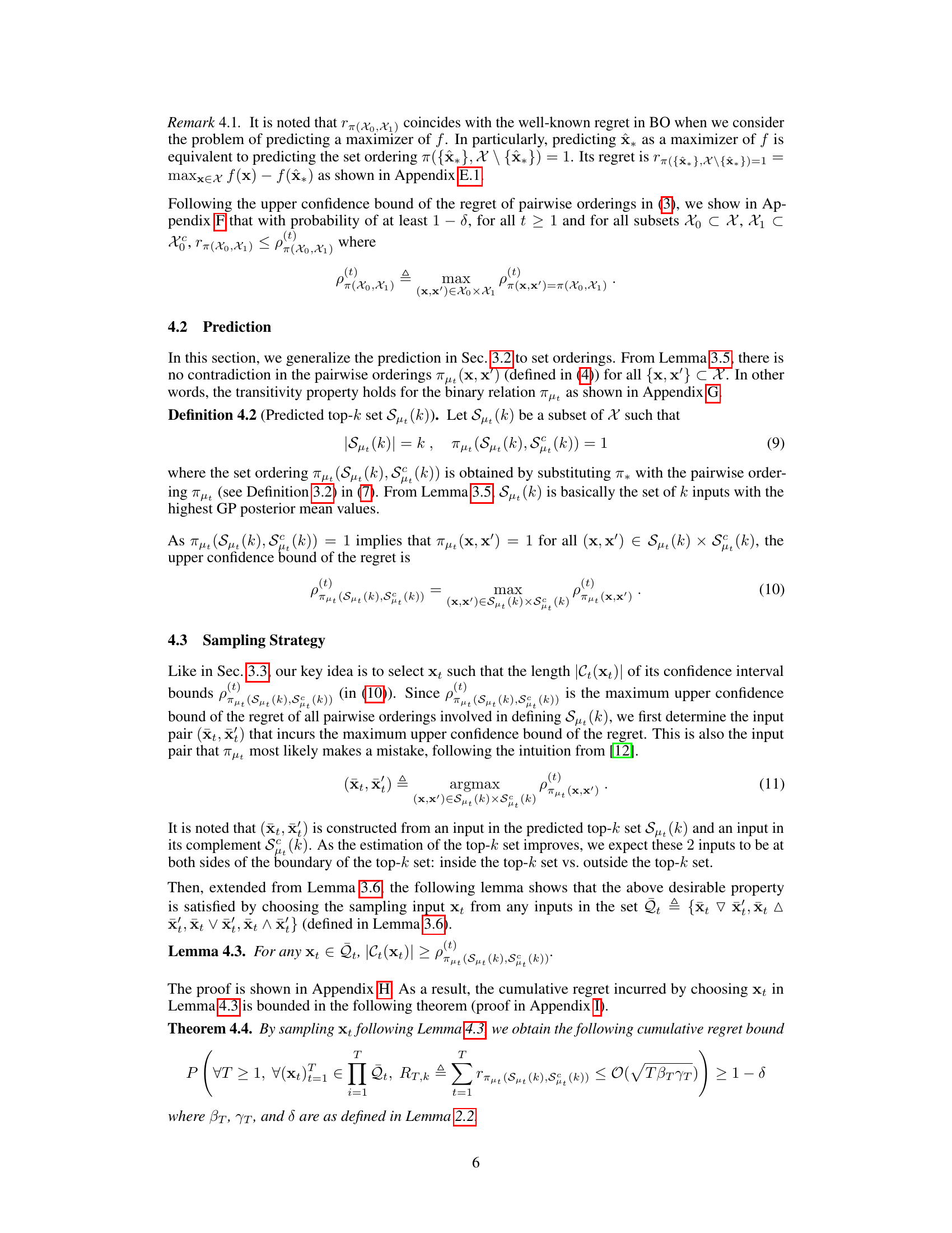
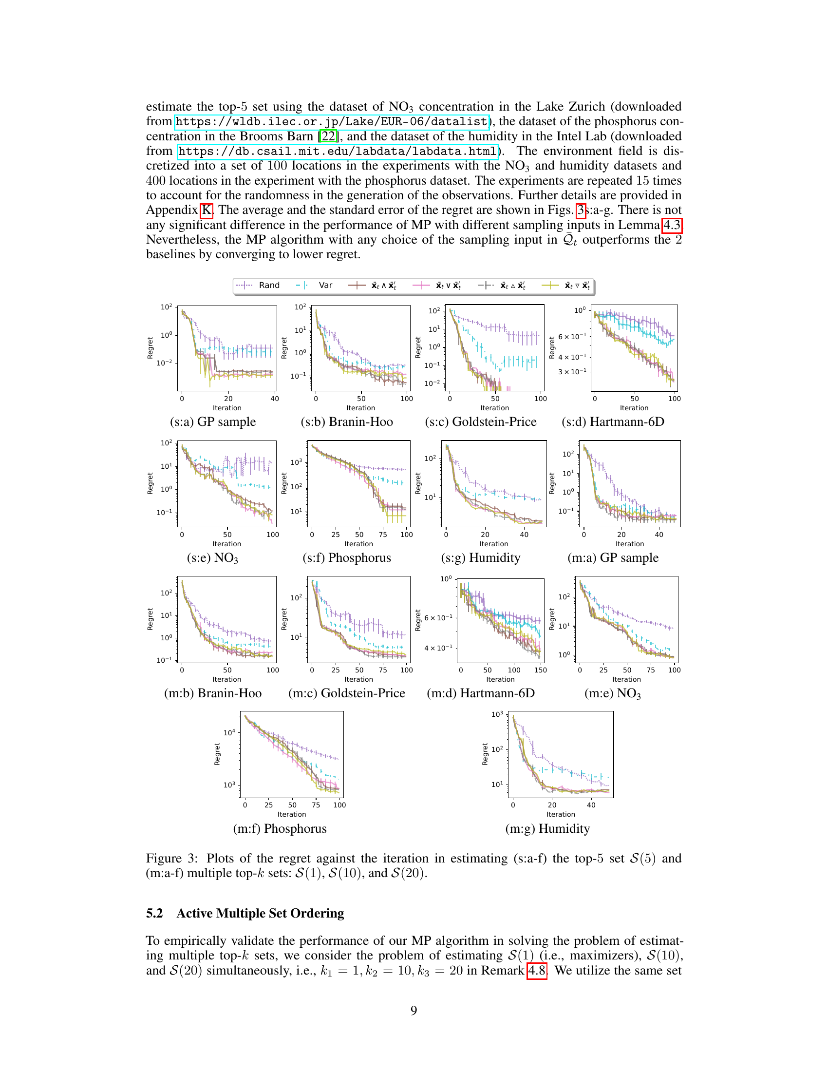
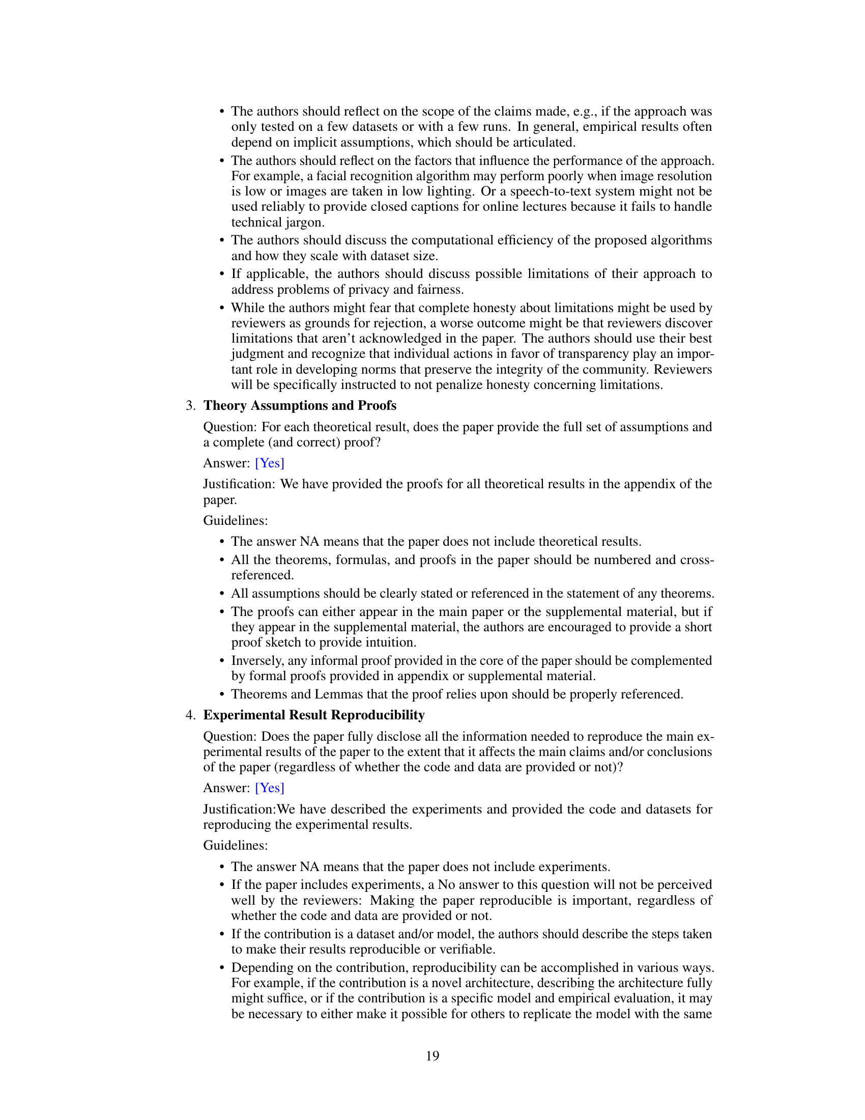
🔼 This figure compares the performance of the Mean Prediction (MP) algorithm with different sampling strategies (xt ∈ {xt ∇ x′, xt △ x′, xt ∨ x′, xt ∧ x′}) against three baselines (PI, EI, MES) for solving the Bayesian Optimization problem. The results are shown for four datasets: Branin-Hoo, NO3, Phosphorus, and Humidity. Each plot shows the regret (a measure of error) over a number of iterations. The goal is to observe how the different methods converge to finding the maximizer of the function and how the different sampling strategies within the MP algorithm perform.
read the caption
Figure 4: Plots of the regret of the predicted maximizer against the iteration.
🔼 This figure compares the performance of two algorithms, MP and Var, in estimating the top 20 inputs (S(20)) with the highest function values from a synthetic function. It visually shows the sampling points chosen by each algorithm over 40 iterations. The plot includes the GP posterior mean, upper and lower confidence bounds, and highlights correctly and incorrectly predicted top-20 inputs, as well as missing top-20 inputs. The histograms display the frequency distribution of sampling points selected by each method. The comparison pair (xt, x’) refers to the pair of inputs used to evaluate the active set ordering.
read the caption
Figure 2: Plot of sampling inputs, GP posterior distribution, and the performance of (a) MP and (b) Var in estimating S(20) of a synthetic function. The comparison pair is (xt, x') in (11). The histogram on the horizontal axis shows the frequency of sampling inputs in 40 iterations.
Full paper#
