↗ OpenReview ↗ NeurIPS Homepage ↗ Chat
TL;DR#
Multi-fidelity best-arm identification (MFB-BAI) aims to efficiently find the best option from multiple choices with varying levels of accuracy and cost. Existing methods lack optimality due to loose lower bounds on cost complexity. This research tackles this challenge by introducing a tighter, instance-dependent lower bound. This new bound allows for the development of improved algorithms.
The paper proposes a novel gradient-based algorithm that achieves asymptotically optimal cost complexity. This algorithm demonstrates good empirical performance and provides insights into the concept of optimal fidelity for each arm, which refers to the cost-effective fidelity level for each arm. This significantly improves upon previous methods, offering a more efficient approach to MFB-BAI.
Key Takeaways#
Why does it matter?#
This paper is crucial for researchers working on multi-fidelity best-arm identification problems. It provides a tight lower bound on cost complexity, which is a major improvement over existing bounds. The paper also proposes a computationally efficient algorithm that matches this lower bound asymptotically, offering significant practical advantages. This work advances our understanding of optimal fidelity in such problems, opening new avenues for research and improved algorithm design. It offers valuable insights applicable to many fields needing efficient decision-making under varying costs and data quality, such as A/B testing and hyperparameter optimization.
Visual Insights#

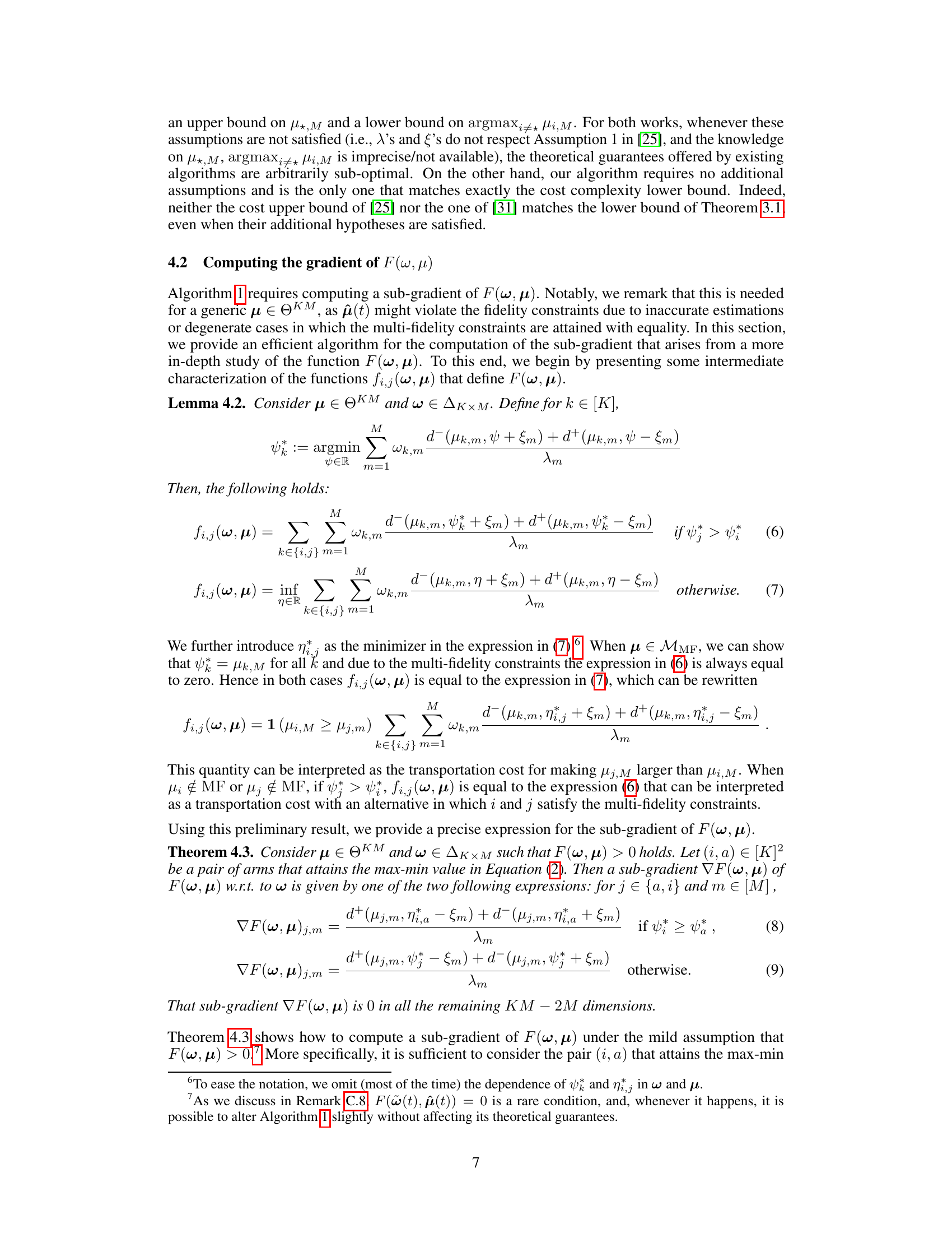
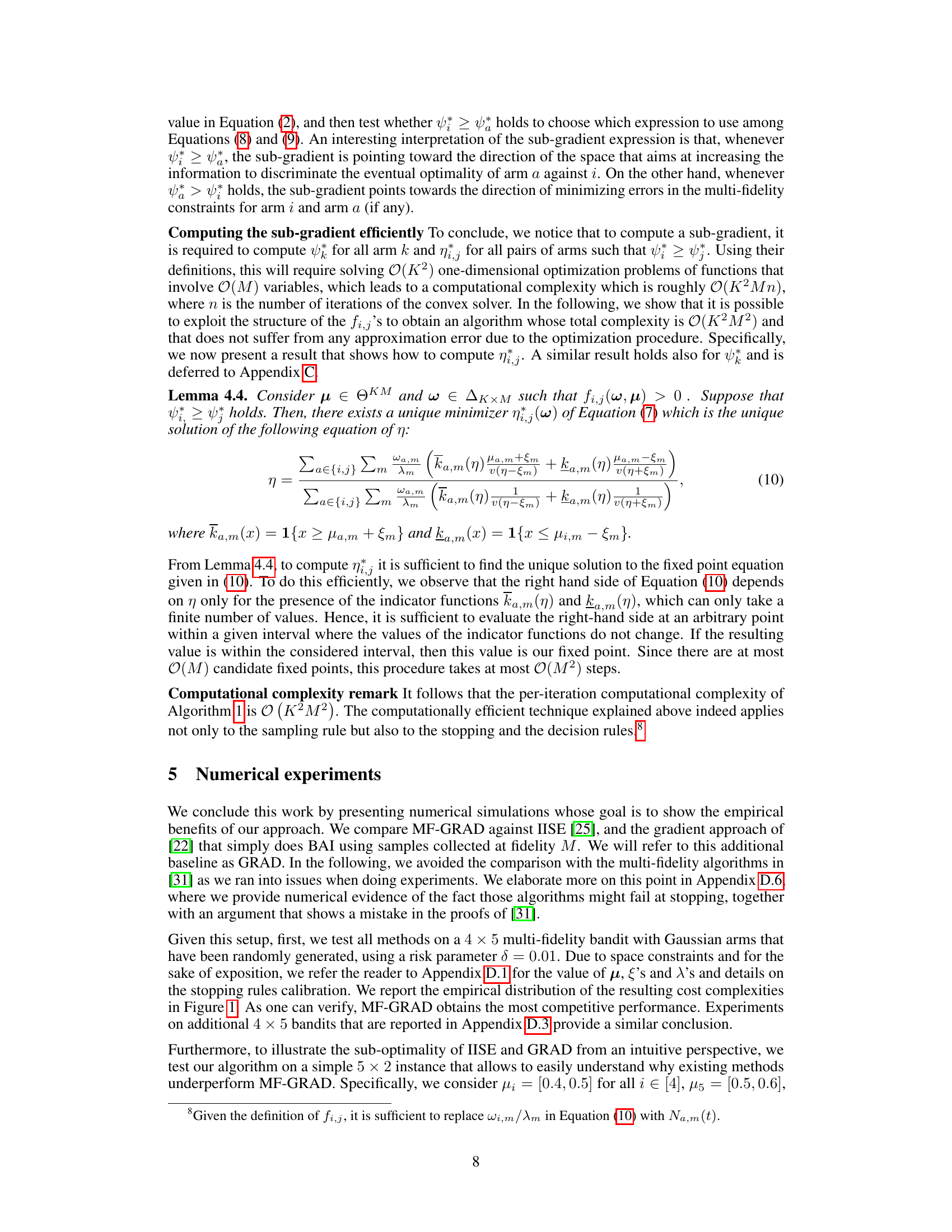
The figure shows the empirical cost complexity results for three different algorithms (GRAD, MF-GRAD, and IISE) across 1000 runs on a 4 × 5 multi-fidelity bandit problem with a risk parameter δ set to 0.01. The boxplots visually represent the distribution of the cost complexities for each algorithm, allowing for a comparison of their performance in terms of the cost required to identify the best arm.

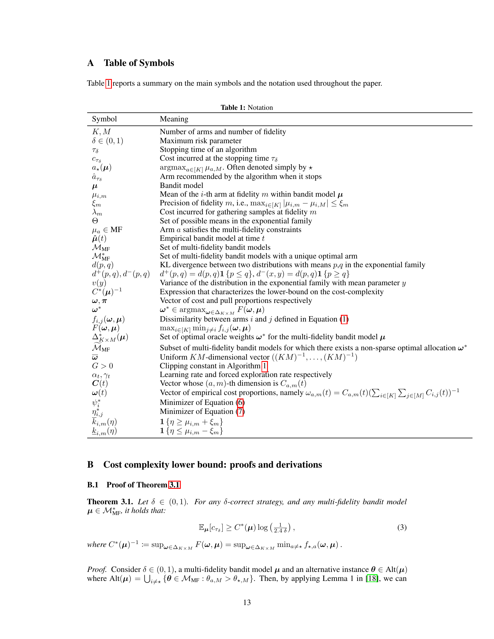
This table lists the notations used throughout the paper. It includes symbols for the number of arms and fidelities, risk parameters, stopping times and costs, the optimal arm, the algorithm’s recommendation, bandit models, means and precisions of observations, fidelity costs, sets of bandit models satisfying multi-fidelity constraints, Kullback-Leibler divergence, variance, and other key mathematical expressions and quantities used in the analysis.
In-depth insights#
MF-BAI Lower Bound#
The heading ‘MF-BAI Lower Bound’ suggests a theoretical investigation into the minimum achievable cost for solving a multi-fidelity best-arm identification (MF-BAI) problem. A lower bound establishes a fundamental limit on performance, indicating that no algorithm can perform better than this limit. The derivation of such a bound likely involves information-theoretic arguments, considering the Kullback-Leibler (KL) divergence between distributions representing different arms and fidelities. The tightness of the bound is crucial, as a loose bound provides limited insight. A tight bound informs the design of optimal or near-optimal algorithms. The lower bound’s dependence on problem parameters, such as arm means and fidelities’ costs and precision, also provides valuable insights. Understanding this dependence helps to characterize the difficulty of specific MF-BAI instances, offering guidance on resource allocation and algorithm design. Finally, comparing the lower bound to the performance of existing algorithms or newly proposed algorithms reveals the algorithms’ optimality. If an algorithm’s performance matches the lower bound asymptotically, it can be considered optimal.
Optimal Fidelity#
The concept of “Optimal Fidelity” in multi-fidelity best-arm identification is crucial for efficient exploration. It represents the ideal balance between the cost and accuracy of information gathered at different fidelity levels. The paper investigates this concept rigorously, establishing a tight instance-dependent lower bound on the cost complexity of any algorithm. This lower bound reveals that each arm might have its own optimal fidelity, implying that a single, globally optimal fidelity does not exist. Furthermore, the lower bound inspires the design of a novel gradient-based algorithm, demonstrating that asymptotically optimal cost complexity is achievable. This algorithm efficiently navigates the fidelity-cost trade-off, outperforming existing methods both theoretically and empirically. The findings highlight that a deeper understanding of optimal fidelity is pivotal for efficient resource allocation and optimal decision-making in multi-fidelity settings.
MF-GRAD Algorithm#
The MF-GRAD algorithm, a novel approach for multi-fidelity best-arm identification, stands out due to its asymptotic optimality. Unlike previous methods, it achieves this without relying on restrictive assumptions or requiring additional prior knowledge about the problem instance. The algorithm cleverly leverages a tight instance-dependent lower bound on the cost complexity, employing a gradient-based approach to efficiently navigate the complex trade-off between information gain and cost at different fidelities. A key insight is the concept of optimal fidelity, suggesting that for each arm, a specific fidelity level provides the best balance of accuracy and cost. While the algorithm doesn’t explicitly identify these optimal fidelities, its asymptotic optimality demonstrates the efficiency of its implicit handling of this trade-off. The computational efficiency of MF-GRAD is another significant advantage, making it a practically viable solution. Empirical results further highlight MF-GRAD’s superior performance compared to existing approaches, particularly in scenarios with a high confidence requirement.
Asymptotic Optimality#
Asymptotic optimality, in the context of multi-fidelity best-arm identification, signifies that an algorithm’s performance approaches the theoretical lower bound on the cost complexity as the confidence parameter (δ) approaches zero. This implies that, given enough resources, the algorithm will find the best arm with a cost that is essentially as low as theoretically possible. The achievement of asymptotic optimality provides a strong guarantee about the algorithm’s efficiency, even though it doesn’t directly translate to finite-sample performance. It’s crucial to note that the actual cost will still depend on the specific problem instance (e.g., the gap between means of arms), and the convergence to optimality might be slow. Therefore, while asymptotic optimality offers a powerful theoretical benchmark, it’s essential to also evaluate an algorithm’s practical efficiency through finite-sample experiments, especially to quantify the impact of problem-specific characteristics on the convergence rate. Moreover, understanding when and how fast asymptotic optimality is achieved is key. This requires thorough analysis of the algorithm and a deep understanding of the trade-offs involved in balancing exploration and exploitation within the multi-fidelity setting. This analysis may include examining the impact of different fidelity levels, the allocation of resources across arms, and the role of sparsity in optimal fidelity allocation.
Empirical Validation#
An Empirical Validation section in a research paper would typically present results from experiments designed to test the paper’s core claims. A strong section would begin by clearly describing the experimental setup, including the datasets used, the metrics employed, and any specific implementation details relevant to reproducibility. The methodology must be rigorous, ensuring that the experiments are well-designed and statistically sound, using appropriate control groups and avoiding potential biases. The presentation of results should be clear and concise, employing appropriate visualizations (graphs, tables, etc.) to highlight key findings. Statistical significance testing is crucial to validate results and demonstrate the reliability of the findings. Finally, a thoughtful discussion of the results should be included, exploring both expected and unexpected outcomes, acknowledging limitations, and relating the findings back to the main hypotheses. A robust empirical validation section is critical for establishing the credibility and impact of a research paper, so any shortcomings can severely impact its reception.
More visual insights#
More on figures

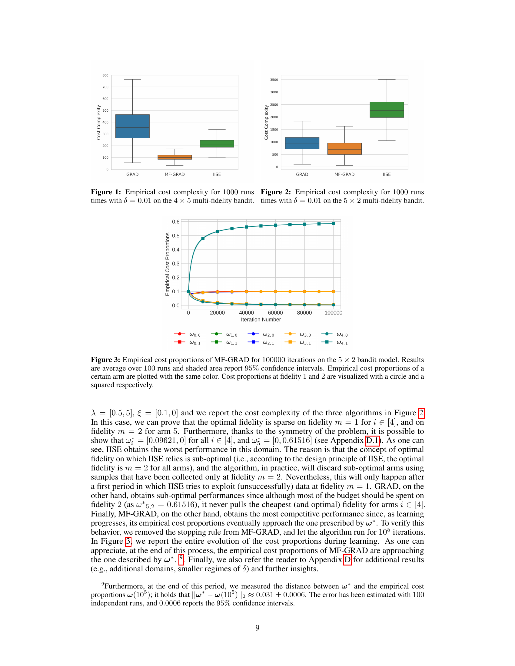
This figure shows the evolution of empirical cost proportions for each arm and fidelity over 100000 iterations of the MF-GRAD algorithm on a 5 × 2 bandit problem. The shaded areas represent 95% confidence intervals, and different colors represent different arms. The plot visualizes how the algorithm dynamically allocates resources across different arms and fidelities, gradually converging towards a sparse optimal allocation.

This figure shows the evolution of empirical cost proportions of MF-GRAD algorithm over 100000 iterations for a 5-arm, 2-fidelity bandit problem. The shaded regions represent 95% confidence intervals, and different colors represent different arms. The plot illustrates how the algorithm dynamically allocates its sampling budget across arms and fidelities, converging towards an optimal allocation.
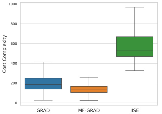
This figure shows the empirical cost complexity (total cost to identify the best arm) for three different algorithms: GRAD, MF-GRAD, and IISE. The experiment was conducted 1000 times on a 4 × 5 multi-fidelity bandit problem with a risk parameter (δ) of 0.01. The box plot visualization displays the median, quartiles, and range of the cost complexity values for each algorithm. The figure highlights the performance comparison of the algorithms in terms of cost efficiency in solving a multi-fidelity best-arm identification problem.
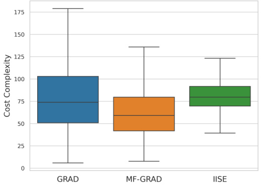
The figure shows the empirical cost complexity (i.e., the total cost incurred until the algorithm stops) for three different algorithms: GRAD, MF-GRAD, and IISE. The box plot shows the distribution of the cost complexity across 1000 independent runs of each algorithm on a 4 × 5 multi-fidelity bandit problem with a risk parameter δ = 0.01. MF-GRAD, the algorithm proposed in this paper, demonstrates significantly lower cost complexity compared to GRAD and IISE.
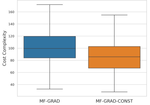
This boxplot compares the cost complexity of MF-GRAD and MF-GRAD-CONST on a 4x5 multi-fidelity bandit problem. MF-GRAD-CONST uses a constant learning rate instead of the theoretical one used in MF-GRAD. The plot shows that MF-GRAD-CONST has a lower median cost complexity and a smaller interquartile range, indicating improved performance with the constant learning rate.
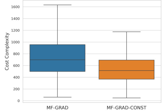
This figure compares the empirical cost complexity of MF-GRAD and MF-GRAD-CONST on the 4 × 5 multi-fidelity bandit problem described in Section 5 of the paper. MF-GRAD-CONST uses a constant learning rate instead of the theoretically derived learning rate used by MF-GRAD. The box plot shows the distribution of costs across the 1000 runs of each algorithm. The results indicate that using a constant learning rate improves the performance of the algorithm, resulting in lower cost complexity.

This figure shows the evolution of the empirical cost proportions of the MF-GRAD algorithm over 100000 iterations on a 5x2 multi-fidelity bandit problem. The shaded areas represent 95% confidence intervals, illustrating the variability in the cost proportions across multiple runs. The plot reveals how the algorithm allocates its budget across different arms and fidelities, highlighting the sparsity pattern of optimal fidelity allocation.
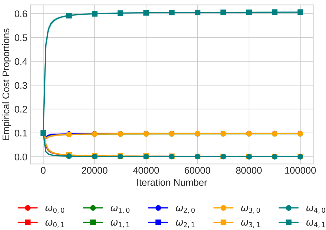
This figure shows the evolution of the empirical cost proportions of the MF-GRAD algorithm over 100000 iterations for a 5 × 2 bandit problem. The results are averaged over 100 runs, and 95% confidence intervals are shown as shaded areas. Each color represents a different arm, and different shapes represent different fidelities.

The figure is a box plot showing the empirical cost complexity results for three algorithms (GRAD, MF-GRAD, IISE) on a 4 × 5 multi-fidelity bandit problem, with a risk parameter δ set to 0.01. Each algorithm is run 1000 times and the box plots summarize the distribution of cost complexities across those runs. The plot visualizes the median, quartiles, and range of the cost complexities for each algorithm, offering a comparison of their performance in terms of the cost required to identify the best arm with the specified confidence.
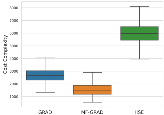
This figure shows the empirical cost complexity (total cost until the algorithm stops) for three different algorithms: GRAD, MF-GRAD, and IISE. Each algorithm is run 1000 times on the same 4x5 multi-fidelity bandit problem (4 arms, 5 fidelities) with a risk parameter δ set to 0.01. The box plots visually represent the distribution of the cost complexities obtained across the 1000 runs for each algorithm, showing the median, quartiles, and outliers. This allows for a comparison of the algorithms’ performance in terms of the total cost required to identify the best arm with a given level of confidence.
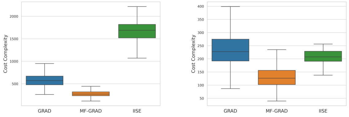
The figure shows the empirical cost complexity of three algorithms (GRAD, MF-GRAD, IISE) for a 4 × 5 multi-fidelity bandit problem, with a risk parameter of δ = 0.01. The boxplot displays the distribution of cost complexities across 1000 independent runs of each algorithm, providing a visual comparison of their performance in terms of cost efficiency. The algorithms differ in their approach to handling multiple fidelities; GRAD uses only the highest fidelity, MF-GRAD is the proposed algorithm which uses a gradient-based approach, and IISE is a previously published algorithm. The plot shows that MF-GRAD is the most cost-effective.
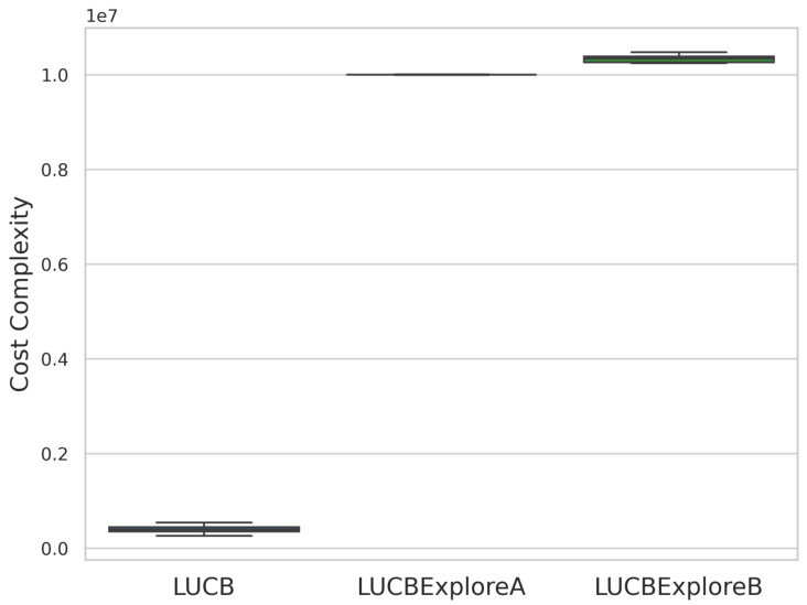
This figure shows the cost complexity of three algorithms, LUCB, LUCBExploreA, and LUCBExploreB. The algorithms were tested on a multi-fidelity bandit problem where the optimal fidelity for each arm is known. The results show that LUCBExploreA and LUCBExploreB fail to terminate within a reasonable time frame (10^7 samples), unlike LUCB which terminates quickly. This highlights a limitation of the LUCBExplore algorithms, specifically their inability to effectively identify the correct fidelity for each arm in all cases, thus leading to non-termination.
More on tables

This table presents the parameter values for a 4x5 multi-fidelity bandit problem used in the paper’s experiments. It shows the mean reward (μ) for each of the four arms (μ₁, μ₂, μ₃, μ₄) at each of the five fidelities (m = 1, 2, 3, 4, 5). The table also includes the maximum bias (ξ) and cost (λ) associated with each fidelity level. This data is used to test and compare the performance of different multi-fidelity best-arm identification algorithms.

This table presents the parameters of a 5 × 2 multi-fidelity bandit problem used in the paper’s numerical experiments. It shows the mean reward (μ) for each of the 5 arms at each of the 2 fidelities (m=1, m=2). The maximal bias (ξ) and the cost (λ) associated with each fidelity are also listed. This specific bandit problem is designed to highlight the benefits of the proposed MF-GRAD algorithm by showcasing a situation where some fidelities are sub-optimal for specific arms. The authors use this example to illustrate how their algorithm outperforms existing approaches by dynamically allocating resources and exploiting the concept of optimal fidelity.

This table presents the parameters for an additional 4x5 multi-fidelity bandit model used in the experiments. It shows the mean reward (μ) for each arm at each fidelity (m), the precision (ξ) of each fidelity, and the cost (λ) associated with each fidelity. This model was generated using a random process similar to the one in the paper’s Appendix D.1, and was used to further validate the performance of the proposed MF-GRAD algorithm compared to existing approaches.

This table presents the parameters for an additional 4x5 multi-fidelity bandit model used in the experiments. It shows the mean reward (μ) for each of the four arms at each of the five fidelities (m=1 to 5), the precision (ξ) at each fidelity, and the cost (λ) associated with each fidelity. This model is different from the model shown in Table 2 and is used to assess the algorithm’s performance on a wider range of problem instances. The means are set so that means of arms are slightly increasing over fidelities, creating a more stationary trend over fidelity than previous models.
Full paper#
