TL;DR#
Thorax disease classification from radiographic images is challenging due to subtle disease areas, localized variations, and noise. While deep learning shows promise, existing methods don’t effectively address the adverse effects of noise and non-disease areas.
This paper introduces Low-Rank Feature Learning (LRFL), a novel method adding low-rank regularization to the training loss. LRFL leverages the Low Frequency Property (LFP), where low-rank projections retain crucial information. Empirically, LRFL significantly improves classification results on standard datasets (NIH ChestX-ray, COVIDx, CheXpert), surpassing current state-of-the-art methods. Theoretically, LRFL is supported by a sharp generalization bound.
Key Takeaways#
Why does it matter?#
This paper is crucial for researchers in medical image analysis and deep learning. It presents a novel, universally applicable method for improving the accuracy of disease classification on noisy medical images. The method’s strong theoretical foundation and significant performance gains over state-of-the-art techniques open new avenues for research in low-rank feature learning and self-supervised learning. This work is particularly relevant to researchers facing challenges with noisy medical data and limited annotations.
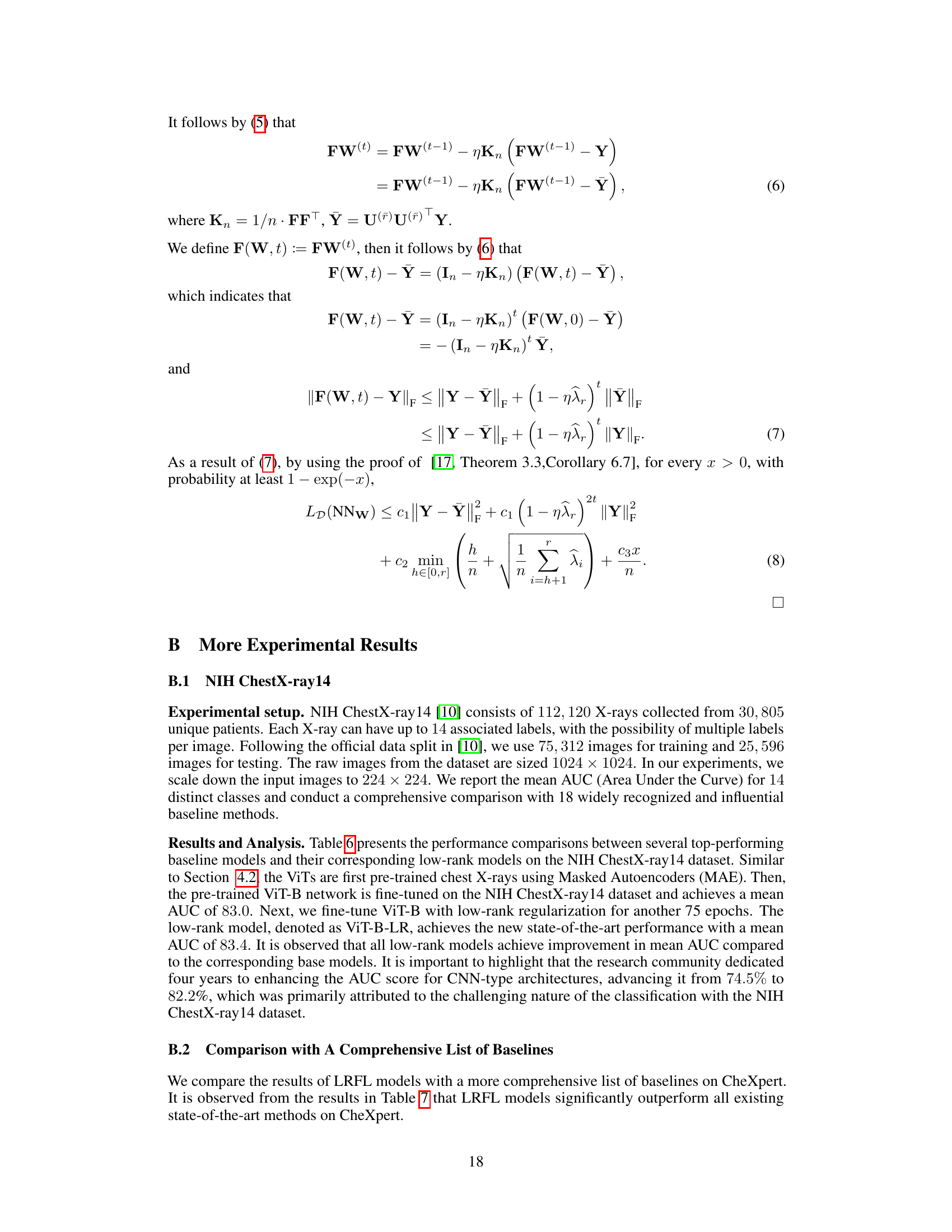
Visual Insights#

🔼 This figure shows the eigen-projection and signal concentration ratio for different ranks on three datasets (NIH ChestXray-14, COVIDx, and CheXpert). It visually demonstrates the Low Frequency Property (LFP), which shows that a low-rank projection of the ground truth training class labels contains most of the information in the original labels. This supports the use of Low-Rank Feature Learning in the paper.
read the caption
Figure 1: Eigen-projection (first row) and signal concentration ratio (second row) of Vit-Base on NiH-ChestXray-14, COVIDx, and CheXpert. To compute the eigen-projection, we first calculate the eigenvectors U of the kernel gram matrix K ∈ Rnxn computed by a feature matrix F ∈ Rnxd, then the projection value is computed by p = ∑=1 || UTY(©) ||2||Y(©)||2 ∈ R, where C is the number of classes, and Y ∈ {0,1}n×C is the one-hot labels of all the training data, Y(c) is the c-th column of Y. The eigen-projection p, for r ∈ [min(n, d)] reflects the amount of the signal projected onto the r-th eigenvector of K, and the signal concentration ratio of a rank r reflects the proportion of signal projected onto the top r eigenvectors of K. The signal concentration ratio for rank r is computed by ||p(1:r) ||2, where p(1:r) contains the first r elements of p. For example, by the rank r = 38, the signal concentration ratio of Y on NIH ChestX-ray14, COVIDx, and CheXpert are 0.959, 0.964, and 0.962 respectively.
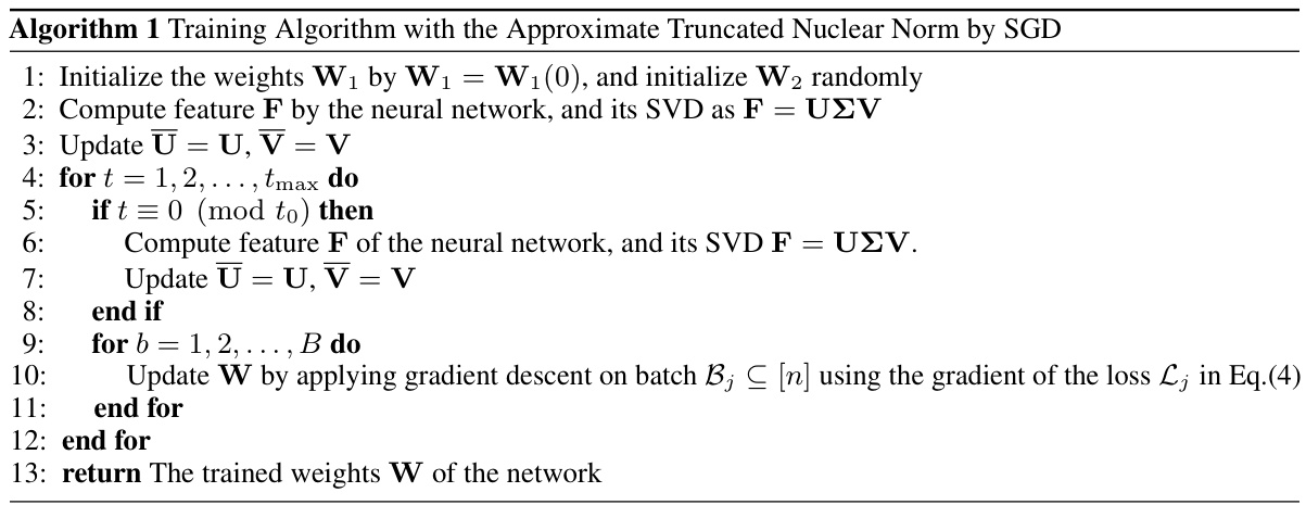
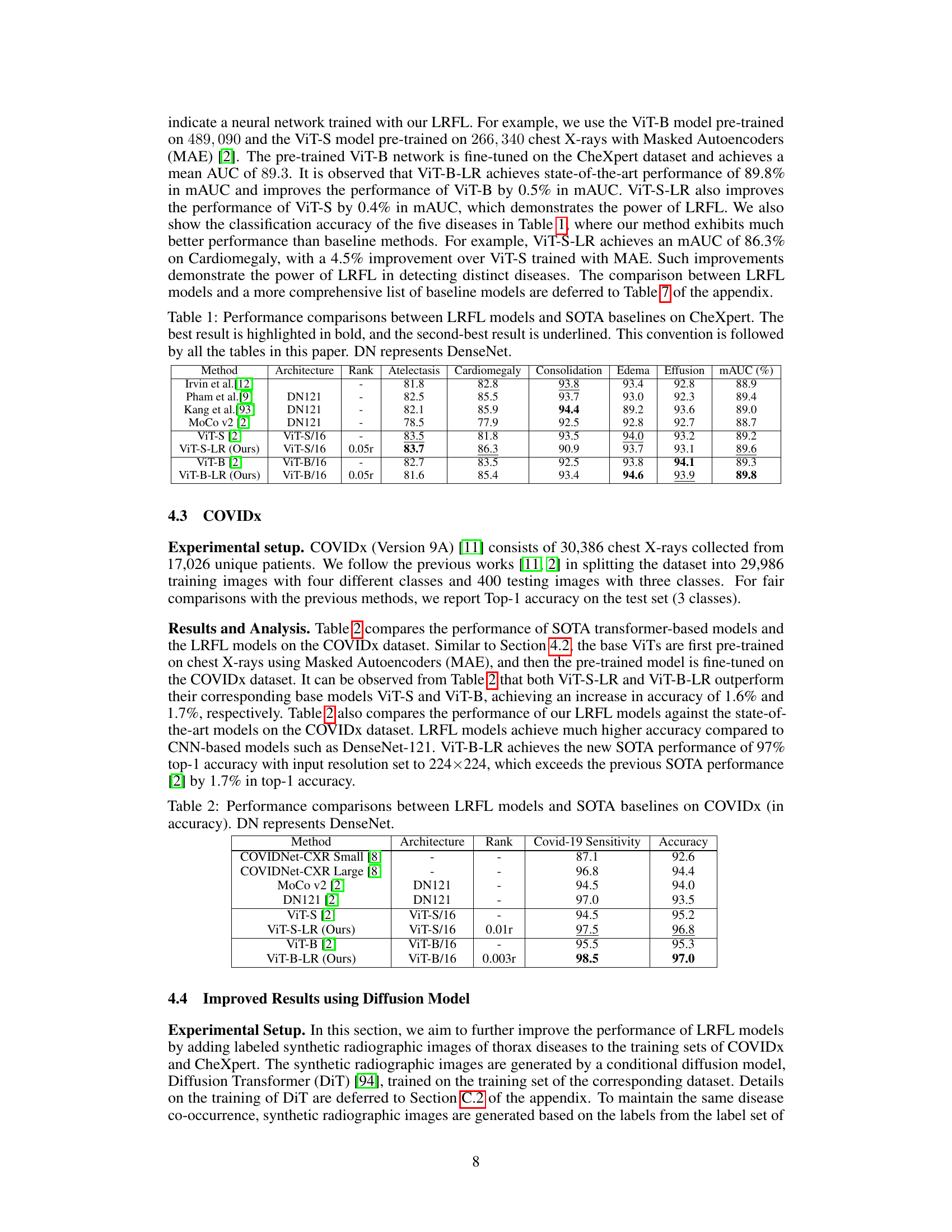
🔼 This table compares the performance of the proposed Low-Rank Feature Learning (LRFL) method with state-of-the-art (SOTA) baselines on the CheXpert dataset for thorax disease classification. It shows the mAUC and accuracy for several diseases, highlighting the improved performance of the LRFL models (ViT-S-LR and ViT-B-LR) over the baseline models (ViT-S and ViT-B). DN refers to DenseNet.
read the caption
Table 1: Performance comparisons between LRFL models and SOTA baselines on CheXpert. The best result is highlighted in bold, and the second-best result is underlined. This convention is followed by all the tables in this paper. DN represents DenseNet.
In-depth insights#
Low-Rank Feature#
The concept of “Low-Rank Feature” learning, as presented in the paper, offers a novel approach to improve the accuracy and robustness of thorax disease classification. The core idea revolves around leveraging the low-frequency property (LFP), which posits that essential information in medical images is primarily concentrated within low-rank components. This property is supported by empirical evidence and theoretical analysis, suggesting that high-rank features frequently incorporate noise and irrelevant background details. By integrating a truncated nuclear norm as a regularization term within the training process, the method effectively filters out such high-rank noise. This low-rank regularization enhances the model’s ability to focus on the crucial, low-rank discriminative features, leading to improved generalization performance and better classification results. The approach’s universality and theoretical grounding suggest its broader applicability beyond thorax disease classification to other medical image analysis tasks.
LRFL Method#
The Low-Rank Feature Learning (LRFL) method, a core contribution of the paper, tackles the challenge of noise and irrelevant background information in medical image classification. It leverages the Low Frequency Property (LFP) observed in deep neural networks and thorax medical datasets, suggesting that low-rank features capture essential disease information. LRFL introduces a low-rank regularization term (truncated nuclear norm) to the neural network’s training loss, effectively suppressing high-rank noise components. This approach is universally applicable to various neural network architectures (CNNs and ViTs). Importantly, the paper presents a novel separable approximation for the truncated nuclear norm, enabling efficient optimization using standard SGD, unlike prior low-rank methods. Empirical results demonstrate LRFL’s superior performance, achieving state-of-the-art results on benchmark thorax disease datasets. The method is theoretically supported by a sharp generalization bound, further solidifying its effectiveness.
Thorax Disease#
The research paper focuses on thorax disease classification, employing deep neural networks to analyze radiographic images. A core challenge addressed is the effective extraction of features from these images, particularly concerning the impact of noise and background interference on accurate disease identification. The paper proposes a novel method, Low-Rank Feature Learning (LRFL), designed to mitigate these issues by focusing on low-rank features which are less susceptible to noise and background variations. This approach is supported by both empirical and theoretical justifications, demonstrating improvements in classification accuracy compared to existing methods. The application of LRFL to various neural network architectures (CNNs and ViTs) across multiple datasets (NIH ChestX-ray, COVIDx, CheXpert) showcases its broad applicability and effectiveness in improving thorax disease classification.
Synthetic Images#
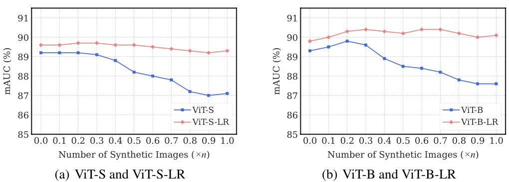
The utilization of synthetic images for augmenting training data in medical image analysis is a crucial aspect of the research. Synthetic data generation offers a way to address the challenges of limited and expensive real-world medical datasets. The paper explores leveraging synthetic images generated by a conditional diffusion model to boost the accuracy of thorax disease classification. This approach is particularly beneficial because it addresses the scarcity of high-quality annotated medical imaging data. The integration of synthetic images is carefully managed to avoid introducing excessive noise and to improve overall model performance. A key contribution of the paper is the demonstration of how the addition of appropriate quantities of synthetic images, determined through cross-validation, improves the performance of the low-rank feature learning (LRFL) models. This innovative use of synthetic data significantly enhances the robustness and generalizability of the models, leading to superior classification results. It showcases how careful selection and integration of synthetic data can effectively overcome limitations in real-world datasets, paving the way for more robust and accurate medical image analysis applications.
Ablation Study#
An ablation study systematically investigates the contribution of individual components within a machine learning model. By removing or altering parts of the model (e.g., layers in a neural network, specific regularization terms, or data augmentation techniques), researchers can isolate the impact of each component on the overall performance. This process is crucial for understanding the model’s behavior, identifying critical elements, and guiding future development. A well-designed ablation study requires careful consideration of the features being removed, the order of removal, and appropriate evaluation metrics. It helps to assess the generalizability of findings, potentially revealing unexpected interactions between components. The results of an ablation study often inform model simplification, enhancing efficiency and interpretability. Furthermore, by highlighting aspects that significantly impact performance, these studies directly contribute to identifying avenues for future improvements and informing design choices for related models.
More visual insights#
More on figures

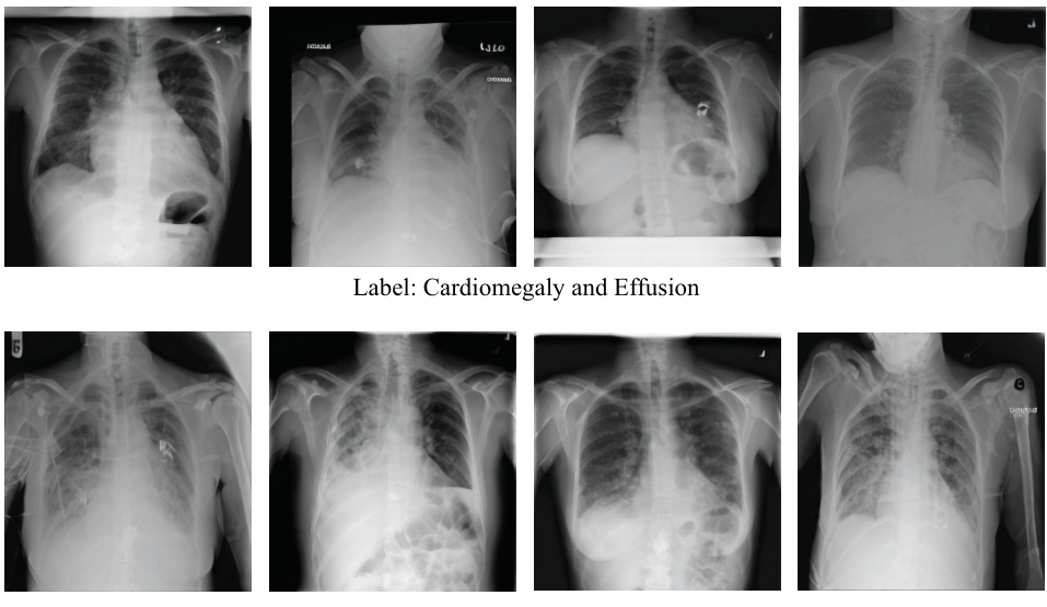
🔼 This figure shows Grad-CAM visualization results for both the ViT-Base and the Low-Rank ViT-Base models on the NIH ChestX-ray14 dataset. Grad-CAM highlights the image regions that are most important to the model’s predictions. The top row displays the ViT-Base model’s attention, while the bottom row shows the Low-Rank ViT-Base’s attention. A comparison reveals that the Low-Rank model focuses more on the disease areas, while the original ViT-Base model also highlights irrelevant background regions.
read the caption
Figure 2: Robust Grad-CAM [95] visualization results on NIH ChestX-ray 14. The figures in the first row are the visualization results of ViT-Base, and the figures in the second row are the visualization results of Low-Rank ViT-Base.

🔼 This figure shows the eigen-projection and signal concentration ratio for different ranks (low-rank features) on three datasets: NIH ChestXray-14, COVIDx, and CheXpert. The eigen-projection illustrates how much of the signal from the class labels is captured by the top eigenvectors of a kernel gram matrix (computed using feature vectors). The signal concentration ratio shows the proportion of signal captured by the top r eigenvectors for different ranks, indicating how much information is contained in low-rank features. The results show that a significant amount of information from the class labels is concentrated in low-rank projections.
read the caption
Figure 1: Eigen-projection (first row) and signal concentration ratio (second row) of Vit-Base on NiH-ChestXray-14, COVIDx, and CheXpert. To compute the eigen-projection, we first calculate the eigenvectors U of the kernel gram matrix K ∈ Rnxn computed by a feature matrix F ∈ Rnxd, then the projection value is computed by p = ∑c=1 ||UTY(c)||2/||Y(c)||2 ∈ R, where C is the number of classes, and Y ∈ {0,1}n×C is the one-hot labels of all the training data, Y(c) is the c-th column of Y. The eigen-projection p, for r ∈ [min(n, d)] reflects the amount of the signal projected onto the r-th eigenvector of K, and the signal concentration ratio of a rank r reflects the proportion of signal projected onto the top r eigenvectors of K. The signal concentration ratio for rank r is computed by ||p(1:r)||2, where p(1:r) contains the first r elements of p. For example, by the rank r = 38, the signal concentration ratio of Y on NIH ChestX-ray14, COVIDx, and CheXpert are 0.959, 0.964, and 0.962 respectively.

🔼 This figure shows the Grad-CAM visualization results for both the baseline ViT-Base model and the proposed Low-Rank ViT-Base model on the NIH ChestX-ray14 dataset. Grad-CAM highlights the regions of the input image that are most important for the model’s predictions. The comparison highlights how the Low-Rank model focuses more precisely on the relevant disease areas within the bounding box, whereas the baseline model shows activations in less relevant areas, suggesting improved robustness to noise and background.
read the caption
Figure 2: Robust Grad-CAM [95] visualization results on NIH ChestX-ray 14. The figures in the first row are the visualization results of ViT-Base, and the figures in the second row are the visualization results of Low-Rank ViT-Base.

🔼 The figure shows Grad-CAM visualization results for both ViT-Base and Low-Rank ViT-Base models on the NIH ChestX-ray14 dataset. Grad-CAM highlights the image regions most influential in the model’s predictions. The comparison aims to illustrate how Low-Rank Feature Learning affects the model’s attention to relevant image areas versus background or noise.
read the caption
Figure 2: Robust Grad-CAM [95] visualization results on NIH ChestX-ray 14. The figures in the first row are the visualization results of ViT-Base, and the figures in the second row are the visualization results of Low-Rank ViT-Base.
🔼 The figure shows eigen-projections and signal concentration ratios for different ranks on three datasets (NIH ChestX-ray14, COVIDx, and CheXpert). Eigen-projections illustrate how much signal from class labels is captured by different eigenvectors from the kernel gram matrix of features. Signal concentration ratios demonstrate the proportion of signal concentrated in the top-ranked eigenvectors. The results support the low-frequency property (LFP), indicating that low-rank features retain most of the class information.
read the caption
Figure 1: Eigen-projection (first row) and signal concentration ratio (second row) of Vit-Base on NiH-ChestXray-14, COVIDx, and CheXpert. To compute the eigen-projection, we first calculate the eigenvectors U of the kernel gram matrix K ∈ Rnxn computed by a feature matrix F ∈ Rnxd, then the projection value is computed by p = ∑c=1 || UTY(c) ||2||Y(c)||2 ∈ R, where C is the number of classes, and Y ∈ {0,1}n×C is the one-hot labels of all the training data, Y(c) is the c-th column of Y. The eigen-projection p, for r ∈ [min(n, d)] reflects the amount of the signal projected onto the r-th eigenvector of K, and the signal concentration ratio of a rank r reflects the proportion of signal projected onto the top r eigenvectors of K. The signal concentration ratio for rank r is computed by ||p(1:r) ||2, where p(1:r) contains the first r elements of p. For example, by the rank r = 38, the signal concentration ratio of Y on NIH ChestX-ray14, COVIDx, and CheXpert are 0.959, 0.964, and 0.962 respectively.
🔼 This figure shows the eigen-projection and signal concentration ratio for different ranks on three datasets (NIH ChestX-ray14, COVIDx, and CheXpert). The eigen-projection illustrates how much of the signal (class label information) is captured by the top-ranked eigenvectors of the kernel gram matrix, calculated from the features extracted by a ViT-Base model. The signal concentration ratio shows the cumulative proportion of the signal captured as the rank increases. The results suggest that a low-rank representation of the features preserves a significant portion of the class label information, supporting the use of low-rank feature learning.
read the caption
Figure 1: Eigen-projection (first row) and signal concentration ratio (second row) of Vit-Base on NiH-ChestXray-14, COVIDx, and CheXpert. To compute the eigen-projection, we first calculate the eigenvectors U of the kernel gram matrix K ∈ Rnxn computed by a feature matrix F ∈ Rnxd, then the projection value is computed by p = ∑c=1 ||UTY(c)||2/||Y(c)||2 ∈ R, where C is the number of classes, and Y ∈ {0,1}n×C is the one-hot labels of all the training data, Y(c) is the c-th column of Y. The eigen-projection p, for r ∈ [min(n, d)] reflects the amount of the signal projected onto the r-th eigenvector of K, and the signal concentration ratio of a rank r reflects the proportion of signal projected onto the top r eigenvectors of K. The signal concentration ratio for rank r is computed by ||p(1:r)||2, where p(1:r) contains the first r elements of p. For example, by the rank r = 38, the signal concentration ratio of Y on NIH ChestX-ray14, COVIDx, and CheXpert are 0.959, 0.964, and 0.962 respectively.
More on tables

🔼 This table compares the performance of the proposed Low-Rank Feature Learning (LRFL) method with several state-of-the-art (SOTA) baselines on the CheXpert dataset for thorax disease classification. It shows the mAUC and Accuracy scores for different diseases (Atelectasis, Cardiomegaly, Consolidation, Edema, Effusion). The best-performing model for each metric is highlighted.
read the caption
Table 1: Performance comparisons between LRFL models and SOTA baselines on CheXpert. The best result is highlighted in bold, and the second-best result is underlined. This convention is followed by all the tables in this paper. DN represents DenseNet.

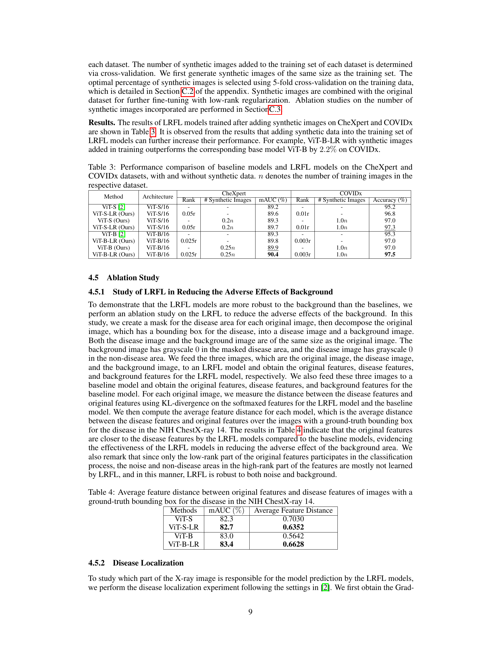
🔼 This table compares the performance of the proposed Low-Rank Feature Learning (LRFL) models with state-of-the-art (SOTA) baselines on the COVIDx dataset. It shows the Covid-19 Sensitivity and Accuracy for different models, including both CNN-based (DenseNet) and Transformer-based (ViT) architectures. The LRFL models consistently outperform their corresponding baselines, demonstrating the effectiveness of the proposed method.
read the caption
Table 2: Performance comparisons between LRFL models and SOTA baselines on COVIDx (in accuracy). DN represents DenseNet.

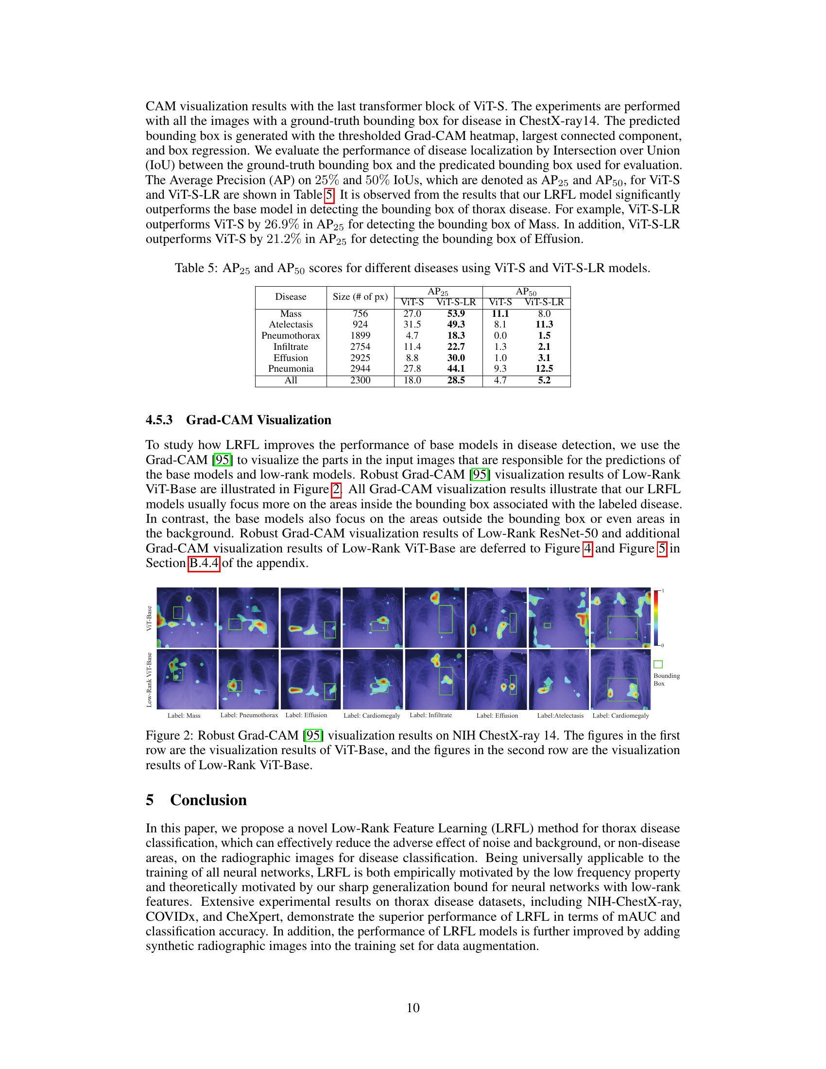
🔼 This table presents a comparison of the performance of baseline models and LRFL models on the CheXpert and COVIDx datasets. It shows the results with and without the addition of synthetic data generated using a diffusion model. The table highlights the improvement in mAUC (multi-class Area Under the Receiver Operating Characteristic Curve) for CheXpert and accuracy for COVIDx achieved by the LRFL models, particularly when augmented with synthetic data.
read the caption
Table 3: Performance comparison of baseline models and LRFL models on the CheXpert and COVIDx datasets, with and without synthetic data. n denotes the number of training images in the respective dataset.

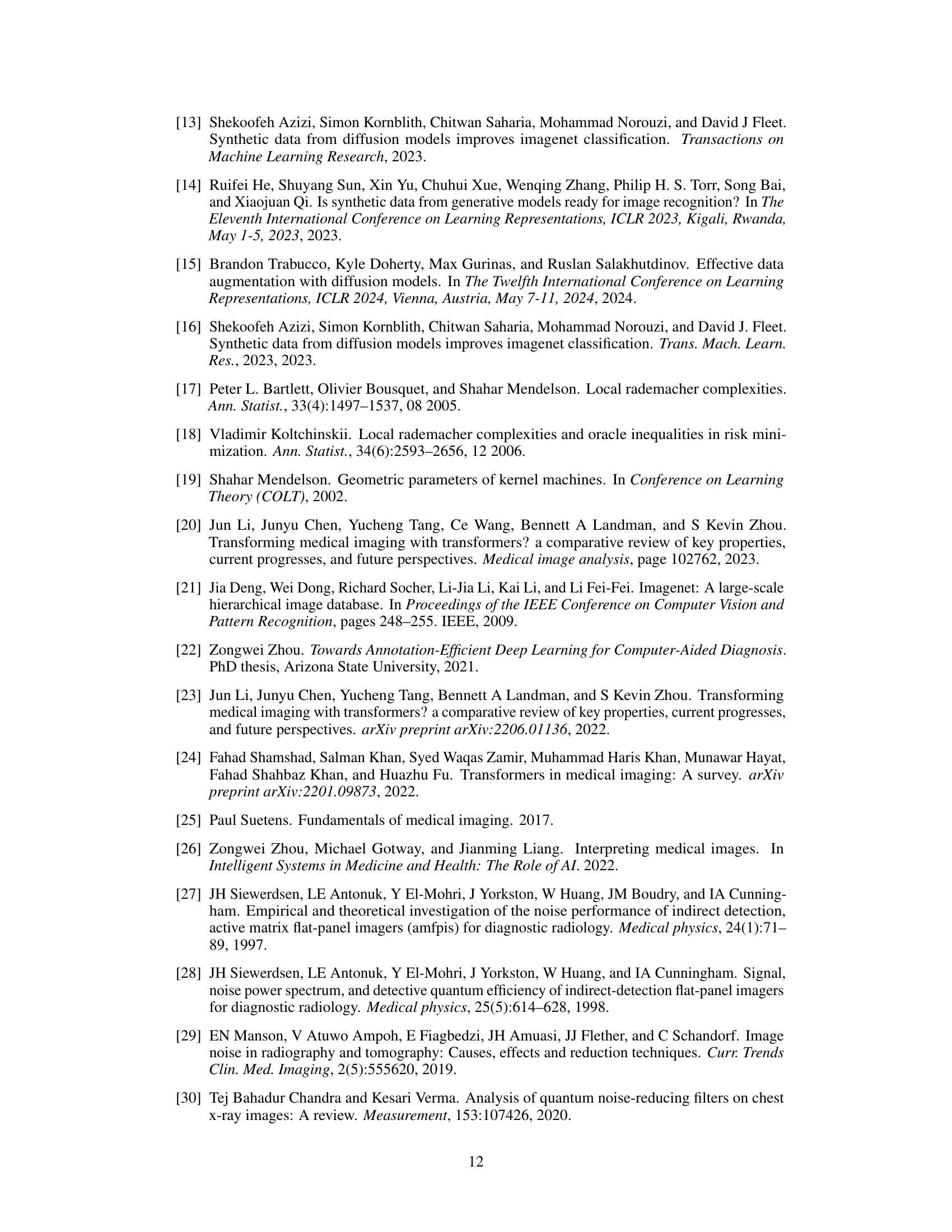
🔼 This table presents a comparison of the average feature distance between original features and disease features for ViT-S, ViT-S-LR, ViT-B, and ViT-B-LR models. The average feature distance is calculated using KL-divergence on the softmaxed features for images in the NIH ChestX-ray14 dataset with ground truth bounding boxes for disease areas. Lower values indicate that the original features are closer to the disease features, suggesting better robustness to background noise.
read the caption
Table 4: Average feature distance between original features and disease features of images with a ground-truth bounding box for the disease in the NIH ChestX-ray 14.

🔼 This table presents the Average Precision (AP) at 25% and 50% Intersection over Union (IoU) for different thorax diseases detected by ViT-S and ViT-S-LR models. It shows that the low-rank feature learning method (LRFL) significantly improves the accuracy of disease localization.
read the caption
Table 5: AP25 and AP50 scores for different diseases using ViT-S and ViT-S-LR models.
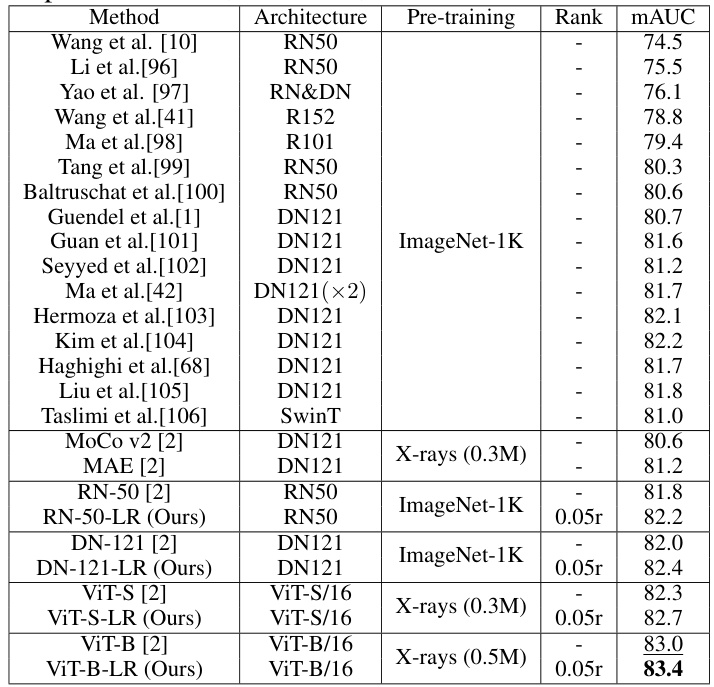
🔼 This table compares the performance of the proposed Low-Rank Feature Learning (LRFL) method with various state-of-the-art (SOTA) methods on the NIH ChestX-ray14 dataset for thorax disease classification. It shows the mAUC scores achieved by different models (ResNet, DenseNet, Swin Transformer, and ViT variants) with and without LRFL. The table highlights the improvement in mAUC achieved by LRFL across different models and pre-training strategies. Pre-training methods include ImageNet-1K and Masked Autoencoders (MAE) on chest X-rays.
read the caption
Table 6: Performance comparisons between LRFL models and SOTA baselines on NIH ChestX-ray14. RN, DN, and SwinT represent ResNet, DenseNet, and Swin Transformer.

🔼 This table compares the performance of the proposed Low-Rank Feature Learning (LRFL) method with several state-of-the-art (SOTA) baseline models on the CheXpert dataset for thorax disease classification. It shows the mAUC and accuracy for each of five diseases (Atelectasis, Cardiomegaly, Consolidation, Edema, and Effusion), as well as the overall mAUC across all five diseases. The best and second-best results are highlighted for easy comparison.
read the caption
Table 1: Performance comparisons between LRFL models and SOTA baselines on CheXpert. The best result is highlighted in bold, and the second-best result is underlined. This convention is followed by all the tables in this paper. DN represents DenseNet.

🔼 This table presents the hyperparameters obtained through cross-validation for different models (ViT-S and ViT-B) on three datasets (NIH ChestX-ray, COVIDx, and CheXpert). The hyperparameters include the rank ratio (γ), the weighting parameter for the truncated nuclear norm (η), and the learning rate (μ). These values were determined using a 5-fold cross-validation process to optimize the performance of the low-rank feature learning method.
read the caption
Table 8: Optimal values of rank ratio γ, weighting parameter η, and learning rate μ decided by cross-validation for different models on different datasets.

🔼 This table presents the time taken for cross-validation on three different datasets (NIH ChestX-ray14, CheXpert, and CovidX) using two different Vision Transformer models (ViT-S-LR and ViT-B-LR). The cross-validation was used to determine optimal hyperparameters (rank ratio γ, weighting parameter η, and learning rate μ) for the LRFL method. The time is reported in minutes for each model and dataset. Note that only 20% of the training data is used for the cross-validation and the models were trained for only 40% of the total training epochs.
read the caption
Table 9: Time Spent for cross-validation on NIH ChestX-ray14, CheXpert, and CovidX. All the results are reported in minutes.

🔼 This table shows the performance of different models (ViT-S, ViT-S-LR, ViT-B, ViT-B-LR) with varying amounts of training data (5%, 10%, 15%, 20%, 25%, 50%) on the NIH ChestX-ray14 dataset. The results demonstrate the effectiveness of the LRFL method in handling small datasets by mitigating overfitting and improving the quality of learned representations.
read the caption
Table 11: The table evaluates the performance of various models under low data regimes on the NIH ChestX-rays14 dataset. Models trained with low-rank features effectively combat overfitting in scenarios with limited data availability, thereby enhancing the quality of representations for downstream tasks.

🔼 This table compares the performance of the proposed Low-Rank Feature Learning (LRFL) method against state-of-the-art (SOTA) baselines on the CheXpert dataset for thorax disease classification. It shows the mAUC and accuracy for several diseases, highlighting the superior performance of LRFL models (ViT-S-LR and ViT-B-LR) compared to the baseline models (ViT-S and ViT-B) and other SOTA methods. The table indicates improvements in both overall mAUC and individual disease classification accuracy for LRFL.
read the caption
Table 1: Performance comparisons between LRFL models and SOTA baselines on CheXpert. The best result is highlighted in bold, and the second-best result is underlined. This convention is followed by all the tables in this paper. DN represents DenseNet.

🔼 This table compares the performance of the proposed Low-Rank Feature Learning (LRFL) models against state-of-the-art (SOTA) baselines on the CheXpert dataset for thorax disease classification. It shows the Area Under the Curve (AUC) and accuracy for multiple diseases, highlighting the superior performance of the LRFL models.
read the caption
Table 1: Performance comparisons between LRFL models and SOTA baselines on CheXpert. The best result is highlighted in bold, and the second-best result is underlined. This convention is followed by all the tables in this paper. DN represents DenseNet.

🔼 This table shows the optimal percentage of synthetic images (α) determined through 5-fold cross-validation for different models and datasets (CheXpert and COVIDx). The optimal percentage of synthetic images that yields the best performance is reported for each model and dataset.
read the caption
Table 14: Selected optimal percentage of images α on different datasets and models.
Full paper#

