TL;DR#
Active learning aims to train machine learning models efficiently by strategically selecting data points to label. Current methods often lack strong theoretical guarantees on convergence rates and sample sizes. The paper addresses this limitation by focusing on both loss-based and uncertainty-based active learning strategies.
This paper proposes a new algorithm called Adaptive-Weight Sampling (AWS) that uses SGD with an adaptive step size. It theoretically analyzes the convergence rate of AWS for smooth convex training loss functions and demonstrates its efficiency through numerical experiments on various datasets. The theoretical analysis provides useful insights into the relationship between sampling strategies, convergence rates, and the number of data points needed. The results show that AWS effectively reduces training time and computational cost compared to other approaches.
Key Takeaways#
Why does it matter?#
This paper is crucial for researchers in machine learning and active learning. It provides rigorous theoretical convergence guarantees for active learning algorithms, something often lacking. The novel Adaptive-Weight Sampling algorithm and its analysis offer practical guidance for algorithm design and data-efficient learning. This work also opens new avenues for future research into loss-based sampling strategies and adaptive step size methods. It is highly relevant to the burgeoning field of efficient machine learning, addressing the growing need for methods that reduce training time and computational cost.
Visual Insights#

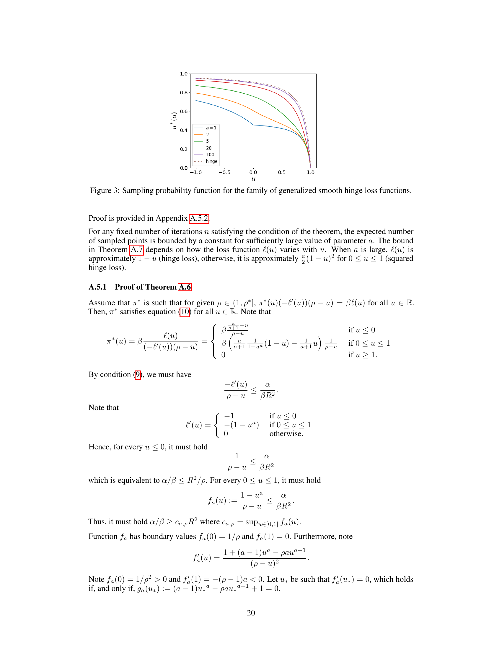
🔼 This figure compares the convergence speed of three different active learning sampling methods: random sampling, loss-based sampling (using absolute error), and the proposed Adaptive-Weight Sampling (AWS) algorithm. The y-axis represents the average cross-entropy loss (a measure of model error), and the x-axis represents the number of iterations. The results visually demonstrate that the AWS algorithm converges faster and achieves lower loss than the other two methods across various datasets.
read the caption
Figure 1: Convergence in terms of average cross-entropy progressive loss of random sampling, loss-based sampling based on the absolute error loss, and our proposed algorithm (loss-based sampling with stochastic Polyak's step size). Our proposed algorithm outperforms the baselines in most cases.

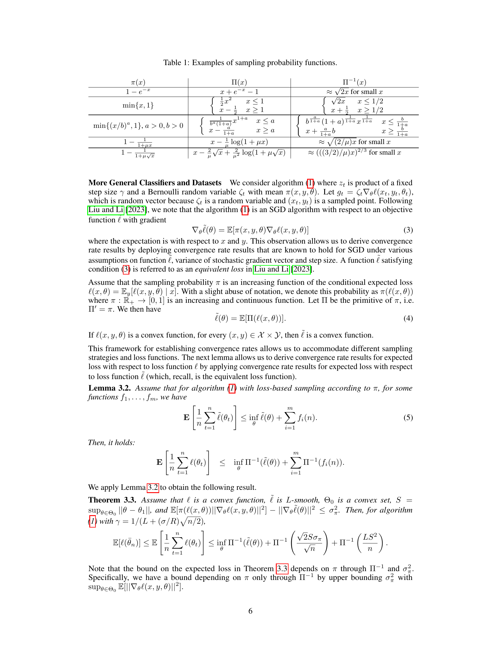
🔼 This table presents examples of sampling probability functions π(x) and their corresponding primitive functions Π(x) and inverse functions Π⁻¹(x). These functions are used in the paper’s analysis of active learning algorithms, where the probability of sampling a data point is related to its loss or uncertainty value. The table shows how various choices of the sampling probability function affect the algorithm’s convergence rate and the expected number of samples. The approximations for small x illustrate the asymptotic behavior of the functions.
read the caption
Table 1: Examples of sampling probability functions.
In-depth insights#
Loss-based Active Learning#
Loss-based active learning represents a paradigm shift in active learning, moving away from solely uncertainty-based sampling. Instead of selecting instances based on their estimated uncertainty, it prioritizes those instances where the model’s predictions are most inaccurate, as measured by a loss function. This approach aligns well with the idea of focusing learning resources on the most informative points. It offers the potential advantage of quicker convergence as compared to uncertainty-based methods, particularly when dealing with complex models or noisy data, but requires careful consideration of loss function selection and unbiased loss estimation. An accurate estimate of the loss function is crucial; otherwise, the algorithm could be misled, choosing uninformative instances for labeling. Furthermore, different loss functions will have different convergence rates and sample complexities, hence the choice must be aligned with the specifics of the problem and model. The theoretical analysis and practical application of loss-based active learning necessitate a thorough investigation of these critical aspects to fully realize its potential.
SGD Convergence Rates#
The convergence rate of stochastic gradient descent (SGD) is a crucial aspect of its efficiency and effectiveness in training machine learning models. The rate determines how quickly the algorithm approaches an optimal solution, impacting computational cost and overall training time. Analyses often focus on factors influencing this rate such as step size selection, the properties of the loss function (e.g., convexity, smoothness), and the characteristics of the data (e.g., separability, dimensionality). Understanding these relationships is vital for optimizing SGD’s performance. Constant step-size analyses often yield O(1/n) convergence rates, where n is the number of iterations, but this can be improved with adaptive step sizes. Advanced analyses might consider non-asymptotic bounds and quantify convergence across various types of loss functions and data distributions, providing more practically useful insights for model training.
Adaptive Sampling AWS#
The proposed Adaptive Weight Sampling (AWS) algorithm represents a novel approach to active learning by integrating adaptive sampling with stochastic gradient descent (SGD). AWS dynamically adjusts the sampling probability of data points based on their estimated loss or uncertainty, prioritizing informative samples for model updates. This adaptive strategy deviates from traditional active learning methods that use fixed sampling rates, leading to potential improvements in efficiency and convergence. By achieving stochastic Polyak’s step size in expectation, AWS offers a theoretically grounded method with established convergence rate guarantees. The algorithm’s effectiveness is supported by numerical experiments demonstrating superior efficiency across various datasets when compared to standard SGD and other loss-based or uncertainty-based active learning techniques. A key strength of AWS lies in its adaptability to different loss functions and sampling strategies, making it a flexible and potentially powerful tool for various machine learning tasks. However, further research is needed to explore the algorithm’s robustness to noisy loss estimators and its performance in high-dimensional spaces.
Numerical Experiments#
The section on Numerical Experiments is crucial for validating the theoretical claims of the research paper. It should thoroughly detail the datasets used, clearly describing their characteristics and relevance to the problem. The evaluation metrics employed should be explicitly defined and justified. A comparison against strong baselines is essential, demonstrating the proposed algorithm’s advantages. The experimental setup needs meticulous explanation, including parameter choices, training procedures, and any preprocessing steps. Error bars or statistical significance tests are necessary to ensure the results’ reliability and to prevent overfitting. The presentation of the results, ideally through clear visualizations, should facilitate understanding. Reproducibility is paramount, so all the necessary information to repeat the experiments should be included, promoting transparency and verifiability of findings. Finally, a discussion interpreting the results relative to the theoretical analysis, acknowledging any limitations and providing future research directions, is expected.
Future Research#
The paper’s “Future Research” section hints at several promising avenues. Tightening convergence rate bounds for both constant and adaptive step-size SGD, particularly under relaxed assumptions on the loss function, is a key goal. A deeper investigation into the impact of biased or noisy loss estimators on convergence is also warranted. Extending the analysis to more complex classifiers beyond linear models and linearly separable datasets is crucial for broader applicability. The study of different sampling strategies and the development of more sophisticated methods for handling loss functions with non-smooth gradients would also be valuable.
More visual insights#
More on figures
🔼 This figure compares the performance of three different sampling methods: random sampling, loss-based sampling using absolute error, and the proposed Adaptive-Weight Sampling (AWS) algorithm, in terms of average cross-entropy progressive loss. Progressive loss is calculated sequentially on each datapoint. The x-axis represents the number of iterations, and the y-axis represents the average cross-entropy loss. The AWS method consistently shows lower loss than the other two, demonstrating its superior performance.
read the caption
Figure 1: Convergence in terms of average cross-entropy progressive loss of random sampling, loss-based sampling based on the absolute error loss, and our proposed algorithm (loss-based sampling with stochastic Polyak's step size). Our proposed algorithm outperforms the baselines in most cases.
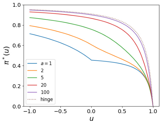
🔼 This figure shows the sampling probability function π* for different values of the parameter a in the generalized smooth hinge loss function. The parameter a controls the smoothness of the hinge loss function, with larger values of a resulting in smoother functions that approach the standard hinge loss function as a goes to infinity. The plot demonstrates that as the value of a increases, the sampling probability function π* becomes increasingly concave, approaching the behavior of the standard hinge loss function as a approaches infinity.
read the caption
Figure 3: Sampling probability function for the family of generalized smooth hinge loss functions.

🔼 This figure compares the performance of three different sampling methods for active learning: random sampling, loss-based sampling (using the absolute error loss), and the proposed Adaptive-Weight Sampling (AWS) algorithm. The y-axis represents the average cross-entropy progressive loss, while the x-axis shows the number of iterations. The results demonstrate that the AWS algorithm consistently achieves lower loss than the other two methods across various datasets, showcasing its efficiency in active learning.
read the caption
Figure 1: Convergence in terms of average cross-entropy progressive loss of random sampling, loss-based sampling based on the absolute error loss, and our proposed algorithm (loss-based sampling with stochastic Polyak's step size). Our proposed algorithm outperforms the baselines in most cases.

🔼 This figure demonstrates the efficiency of different sampling methods in active learning. The x-axis represents the labeling cost (number of labeled instances used for training), and the y-axis represents the average cross-entropy loss. Three sampling strategies are compared: random sampling, loss-based sampling (proportional to absolute error loss), and the proposed Adaptive-Weight Sampling (AWS-PA) algorithm. The results show that AWS-PA outperforms both random and loss-based sampling, achieving lower cross-entropy loss at the same labeling cost. This indicates that AWS-PA effectively selects more informative samples for training, leading to faster convergence and higher model accuracy.
read the caption
Figure 5: Average cross entropy loss as a function of labeling cost for different sampling methods.

🔼 This figure compares the convergence rate of three different active learning algorithms: random sampling, loss-based sampling (using absolute error), and the proposed Adaptive-Weight Sampling (AWS) algorithm. The y-axis shows the average cross-entropy progressive loss, which is a measure of how well the model is learning over time. The x-axis represents the number of iterations. The AWS algorithm consistently shows faster convergence than the other methods, indicating its improved efficiency in active learning.
read the caption
Figure 1: Convergence in terms of average cross-entropy progressive loss of random sampling, loss-based sampling based on the absolute error loss, and our proposed algorithm (loss-based sampling with stochastic Polyak's step size). Our proposed algorithm outperforms the baselines in most cases.

🔼 The figure compares the performance of three different sampling methods: random sampling, loss-based sampling (absloss), and the proposed Adaptive-Weight Sampling (AWS-PA) algorithm. The y-axis represents the average cross-entropy progressive loss, which measures the model’s error during training. The x-axis shows the number of iterations or data points processed. The plot shows that AWS-PA consistently achieves lower loss than the other two methods, indicating its superior efficiency in learning from a limited set of labeled data.
read the caption
Figure 1: Convergence in terms of average cross-entropy progressive loss of random sampling, loss-based sampling based on the absolute error loss, and our proposed algorithm (loss-based sampling with stochastic Polyak's step size). Our proposed algorithm outperforms the baselines in most cases.
🔼 This figure compares the performance of three different sampling methods for active learning: random sampling, loss-based sampling (using absolute error), and the proposed Adaptive-Weight Sampling (AWS) algorithm. The y-axis represents the average cross-entropy loss, and the x-axis represents the number of iterations. The results show that AWS consistently achieves lower loss values than the other two methods across six different datasets, demonstrating its improved efficiency.
read the caption
Figure 1: Convergence in terms of average cross-entropy progressive loss of random sampling, loss-based sampling based on the absolute error loss, and our proposed algorithm (loss-based sampling with stochastic Polyak's step size). Our proposed algorithm outperforms the baselines in most cases.
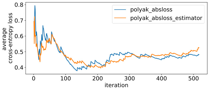
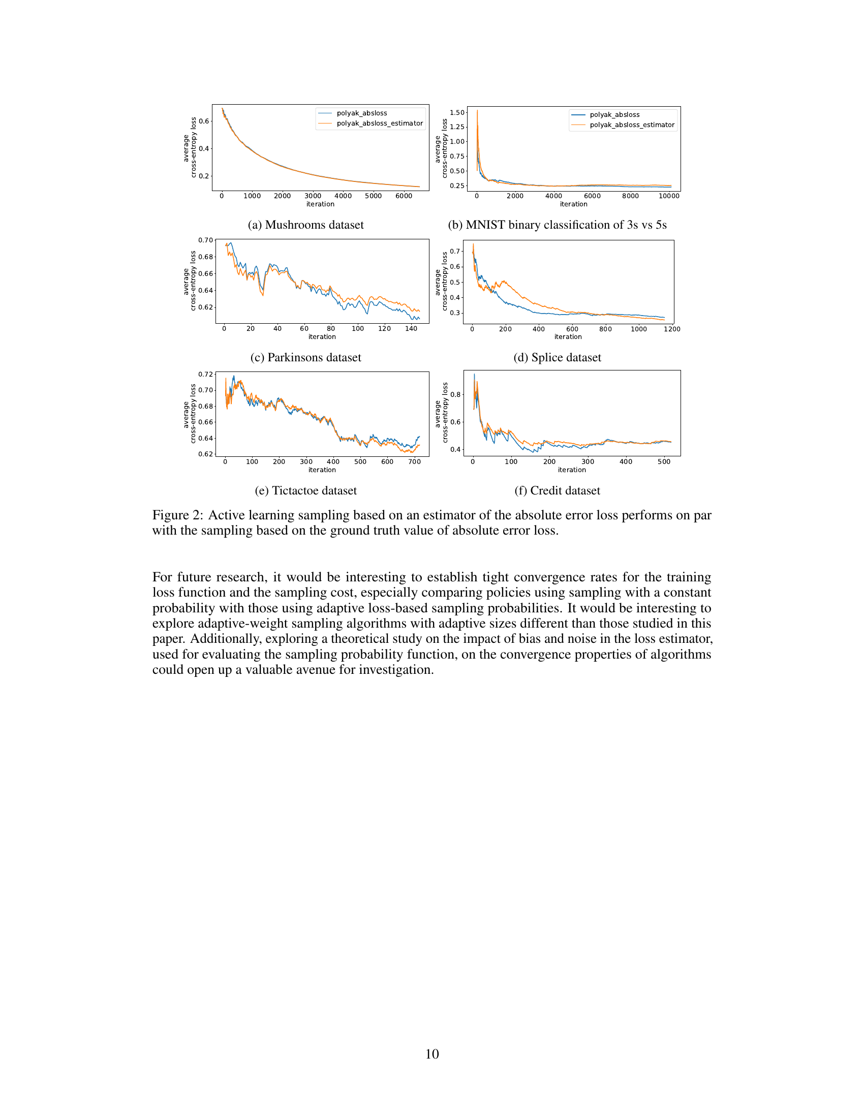
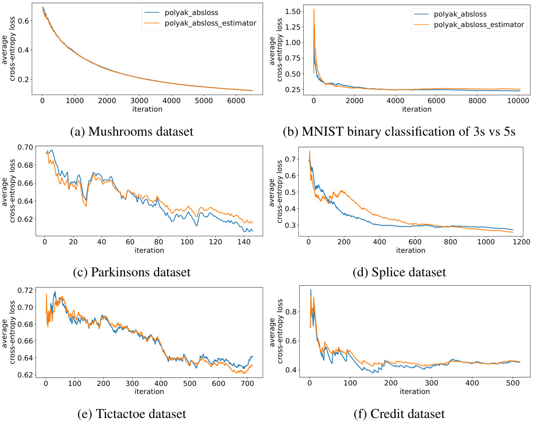
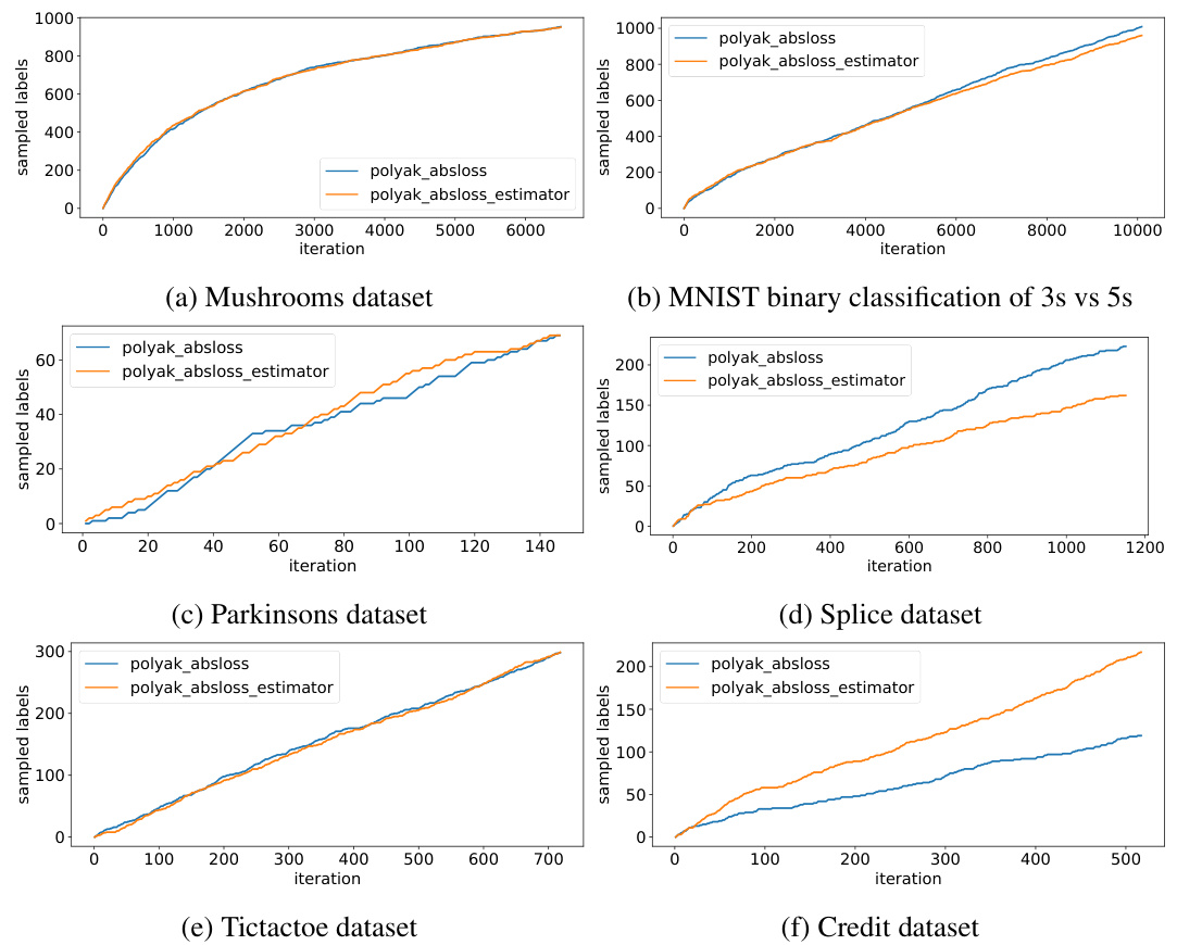
🔼 This figure compares the performance of active learning using two different methods for estimating the absolute error loss: one using the ground truth value and the other using an estimator. The results show that the estimator performs similarly to using the ground truth loss values across six different datasets. The graph plots the average cross-entropy loss against the number of iterations, visualizing how both methods converge over time. This suggests that using an estimator for the loss does not significantly impede the performance of the active learning algorithm.
read the caption
Figure 2: Active learning sampling based on an estimator of the absolute error loss performs on par with the sampling based on the ground truth value of absolute error loss.

🔼 This figure compares the convergence speed of two different optimization methods: SGD with a constant step size and SGD with Polyak’s step size. The experiment is conducted on a subset of the mushrooms dataset, with only 1% and 10% of the data being sampled at each iteration. The graph shows the average cross-entropy loss over iterations. The results demonstrate that using Polyak’s step size leads to faster convergence compared to using a constant step size, even when the amount of data used for training is considerably limited.
read the caption
Figure 10: Average cross-entropy progressive loss of Polyak's step size compared to SGD with constant step size, for 1% and 10% sampling from the mushrooms data.

🔼 This figure shows the robustness of the proposed Adaptive-Weight Sampling algorithm against the noise in the absolute error loss estimator. The y-axis represents the average cross-entropy loss, and the x-axis represents the number of iterations. Four lines are plotted representing different noise levels in the estimator, controlled by parameter ‘a’: high noise (a=1), medium noise (a=2.5), low noise (a=100), and no noise (a=∞, the baseline). The results demonstrate that the algorithm remains effective even with considerable noise in the loss estimation.
read the caption
Figure 11: Robustness of the proposed sampling approach with adaptive Polyak’s step size for different variance var[labs] = labs(1 − labs)/(a + labs) noise levels of absolute error loss estimator: (low) a = 100, (medium) a = 2.5, and (high) a = 1.
Full paper#
