↗ OpenReview ↗ NeurIPS Homepage ↗ Chat
TL;DR#
Traditional time series anomaly detection primarily focuses on temporal patterns, often ignoring valuable spatial relationships between features. This limitation can lead to inaccurate anomaly detection and hinder effective diagnosis, particularly in complex systems with intricate interactions. SARAD addresses this by incorporating spatial associations, offering a more comprehensive and nuanced approach.
SARAD uses a Transformer to capture spatial associations between features and a Multi-Layer Perceptron (MLP) to model the changes in these associations over time. This dual-module architecture, combined with a novel subseries division technique, enables robust anomaly detection and diagnosis. Experimental results on real-world datasets demonstrate SARAD’s superior performance compared to state-of-the-art methods, highlighting the effectiveness of incorporating spatial information.
Key Takeaways#
Why does it matter?#
This paper is crucial for researchers working on anomaly detection in multivariate time series, especially those focusing on industrial applications. It offers a novel approach that significantly improves detection accuracy and provides valuable insights into the spatial relationships between features, bridging the gap between temporal and spatial modeling. The experimental results demonstrating state-of-the-art performance on real-world benchmarks make this a highly impactful work, opening new avenues for research and development.
Visual Insights#

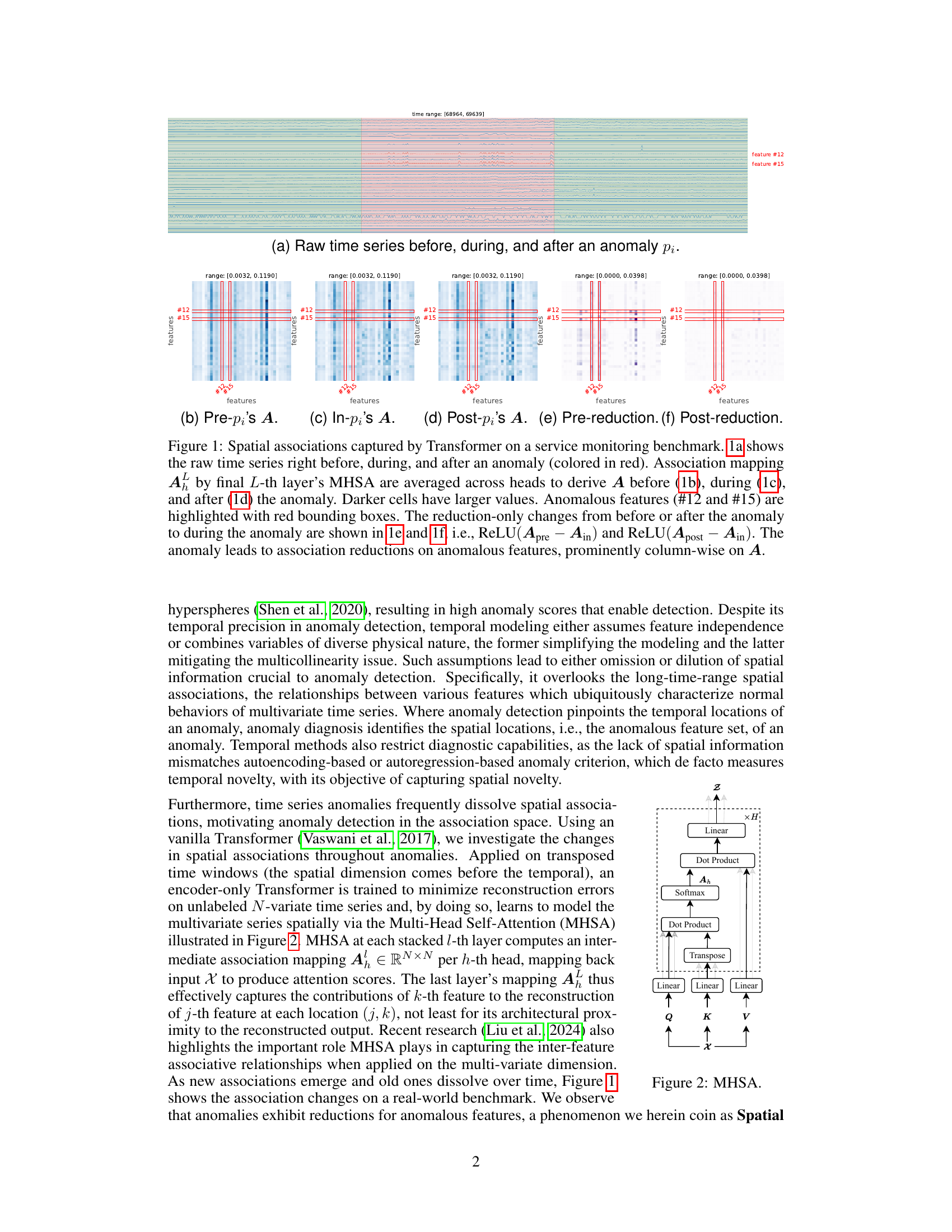
This figure shows how a Transformer model captures spatial associations in a multivariate time series, specifically focusing on changes before, during, and after an anomaly. The raw time series data is displayed alongside visualizations of the association mapping (A) which represents the relationships between features. Changes in these associations are highlighted, demonstrating how anomalies affect these relationships and lead to association reductions, particularly impacting the anomalous features.
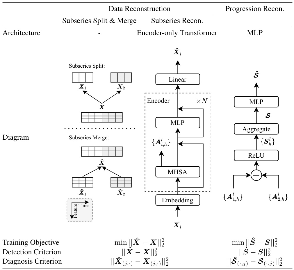
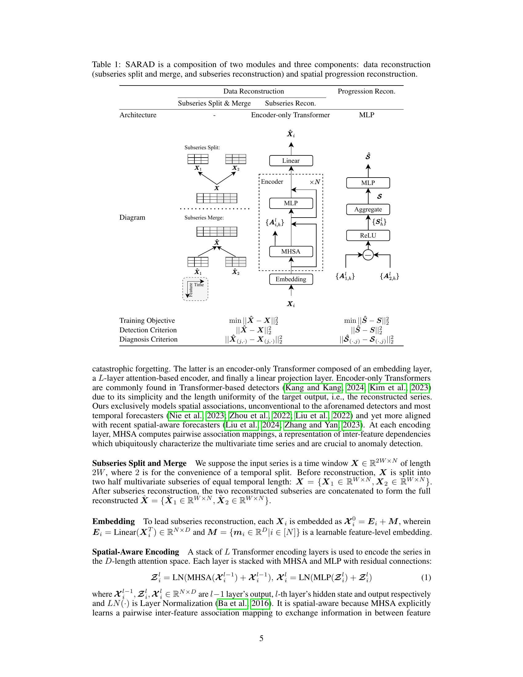
This table summarizes the architecture of the SARAD model, which consists of two main modules: data reconstruction and spatial progression reconstruction. The data reconstruction module uses a subseries split and merge approach with an encoder-only transformer to learn spatial associations. The spatial progression reconstruction module uses an MLP to quantify anomalous association reduction. The table also outlines the training objective and criteria for detection and diagnosis.
In-depth insights#
Spatial Anomaly Detection#
Spatial anomaly detection tackles the challenge of identifying unusual patterns in data with spatial relationships. Unlike temporal methods focusing solely on time series, spatial approaches consider the interconnectedness of data points in space, improving anomaly identification accuracy. This is crucial in applications with geographical data, sensor networks, or image analysis where spatial context is essential. A key advantage is the ability to detect anomalies that might be missed by temporal methods alone, such as localized clusters or geographically spread events. However, the computational complexity can increase significantly with higher dimensionality or denser spatial data. Effective techniques leverage graph-based methods, spatial autoencoders, or deep learning architectures to capture spatial dependencies and effectively distinguish normal from anomalous spatial variations. Future research may focus on developing more efficient algorithms that scale to larger datasets, incorporating multi-modal data sources, and handling dynamic spatial structures.
Transformer-based Encoding#
Transformer-based encoding leverages the power of Transformer networks to learn intricate relationships within multivariate time series data. The core idea is to represent each time step as a sequence of features, allowing the Transformer to capture both temporal and spatial dependencies. This approach goes beyond traditional methods that primarily focus on temporal modeling by explicitly considering how features interact with each other. The self-attention mechanism within the Transformer is particularly crucial, as it enables the model to weigh the importance of different features in relation to each other for a given time step. By learning these spatial associations, the Transformer-based encoder can effectively represent complex interactions within the data, improving anomaly detection and diagnosis accuracy. The effectiveness of this approach is further enhanced by techniques such as subseries division, which helps capture the dynamic nature of these relationships over time. Ultimately, this encoding strategy provides a more nuanced and comprehensive representation of the time series suitable for downstream analysis tasks.
Association Reduction#
The concept of “Association Reduction” presents a novel perspective on anomaly detection in multivariate time series. Instead of solely focusing on temporal patterns, it leverages the disruption of spatial relationships between features as a key indicator of anomalous events. This disruption manifests as a reduction in the strength of associations between features, a phenomenon the authors term “Spatial Association Reduction (SAR)”. The core idea is that anomalies, by their very nature, are unexpected deviations from normal system behavior. This unexpectedness leads to a weakening or breaking of the previously established relationships between data points. SARAD capitalizes on this by employing a Transformer architecture to learn the normal associations between features. Anomalies are then detected by identifying deviations from these learned associations, focusing particularly on column-wise reductions in the association matrix. This approach offers a nuanced understanding of anomalies by identifying not only when they occur (temporally) but also which features are involved (spatially), thus facilitating improved anomaly diagnosis. The effectiveness of this approach is further enhanced by the use of subseries division to capture changes in associations over time.
Robust Anomaly Diagnosis#
Robust anomaly diagnosis in multivariate time series is crucial for effective system monitoring and maintenance. A robust system should not only reliably detect anomalies but also pinpoint their root causes, precisely identifying the anomalous features involved. This requires going beyond simple anomaly scores and delving into the inter-feature relationships that characterize the system’s normal behavior. Successful diagnosis demands the ability to differentiate between genuine anomalous patterns and normal fluctuations that might trigger false alarms. The key lies in leveraging spatial information inherent in the data, capturing the complex interactions between various features. A robust method should also be agnostic to the specific types of anomalies encountered, adapting to diverse data patterns and effectively isolating the anomalous signals even in the presence of noise or confounding factors. Achieving robustness often involves incorporating sophisticated models that can handle the temporal dynamics of multivariate time series and the potential for evolving inter-feature associations, enabling the system to learn and adapt to subtle shifts in normal system behavior while remaining sensitive to genuine anomalies. Ultimately, robust anomaly diagnosis aims to translate raw data into actionable insights for timely intervention, improving overall system reliability and minimizing operational disruption.
SARAD Limitations#
The SARAD model, while demonstrating state-of-the-art performance in multivariate time series anomaly detection and diagnosis, has limitations. A key limitation is its scaling with the number of features; the time complexity is quadratic, leading to significant computational overheads for high-dimensional data. This restricts its applicability to systems with a large number of features. Furthermore, while SARAD effectively leverages spatial information, it relies on the availability of labeled data for diagnosis, which is often scarce and expensive to obtain. The model’s performance might also be affected by the length of anomalies; shorter anomalies in datasets like SMD may prove challenging. Future work should address these issues by exploring techniques such as hierarchical anomaly detection to handle high-dimensionality and developing methods for robust anomaly diagnosis with limited labeled data. The sensitivity of SARAD to hyperparameter choices also needs further study.
More visual insights#
More on figures

This figure shows how the transformer model in SARAD captures spatial associations between features in a multivariate time series. It visualizes these associations as heatmaps (A) before, during, and after an anomaly. The heatmaps illustrate how the relationships between features change due to the anomaly, with darker colors representing stronger associations. The anomalous features are highlighted, and the difference in associations before, during, and after are shown to highlight the anomaly’s impact on the overall feature relationships.

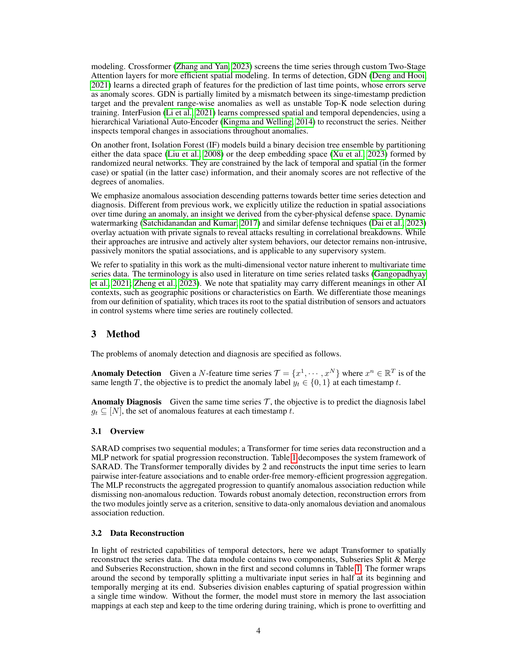
This figure shows the architecture of the Multi-Head Self-Attention (MHSA) mechanism used in the Transformer model. The input is linearly projected into three matrices: Query (Q), Key (K), and Value (V). The dot product of Q and K is computed, followed by a softmax function to generate attention weights. These weights are then used in a dot product with V to produce the output, which is further linearly projected. This process is repeated for multiple heads (H), and the outputs from each head are concatenated.

This figure shows how spatial associations between features change before, during and after an anomaly. The raw time series data shows an anomaly highlighted in red. The association matrix shows the strength of relationships between features (darker means stronger). The anomaly causes a decrease in association, particularly for the anomalous features, as evidenced by the reduction matrices showing the changes in associations compared to during the anomaly.
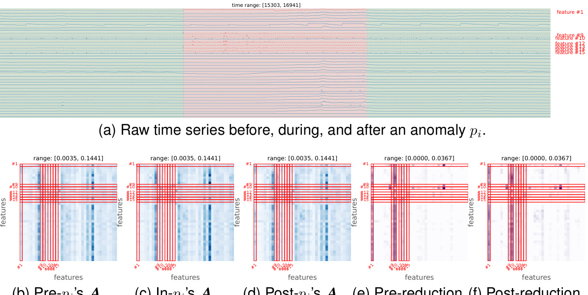
This figure shows how the Transformer model in SARAD captures spatial associations in the SMD dataset before, during, and after an anomaly. Subfigure (a) displays the raw time series data, highlighting the anomaly in red. Subfigures (b), (c), and (d) show the association mappings (A) before, during, and after the anomaly, respectively. Darker cells indicate stronger associations. Subfigures (e) and (f) illustrate the changes in associations (pre-reduction and post-reduction) specifically during the anomaly, showing the reduction in associations as a key characteristic of anomalous events.

This figure shows how a transformer model captures spatial associations in a multivariate time series. The raw time series data is shown alongside the association matrices before, during, and after an anomaly. The matrices highlight how the anomalous features lose their associations with other features during the anomaly, demonstrating the concept of Spatial Association Reduction (SAR).

This figure shows how the transformer captures spatial associations in a service monitoring benchmark. The first subplot shows the raw time series before, during, and after an anomaly. The following subplots show the association mapping before, during and after the anomaly. Darker cells represent stronger associations. The anomalous features are highlighted. Finally, the reduction-only changes to the association mappings are displayed.

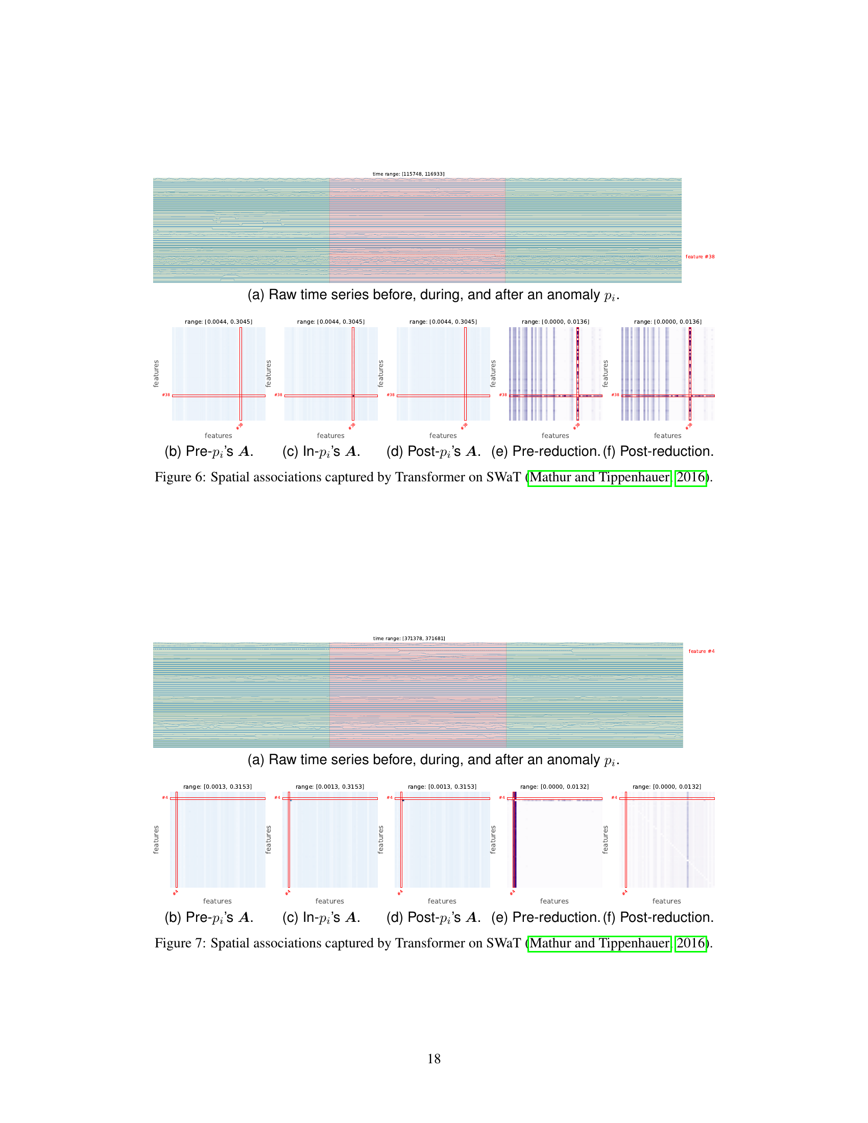
The figure visualizes how spatial associations change before, during, and after an anomaly in the SWaT dataset. Subfigure (a) displays the raw time series, highlighting the anomaly in red. Subfigures (b), (c), and (d) show the association mapping (A) from the Transformer’s Multi-Head Self-Attention (MHSA) layer before, during, and after the anomaly, respectively. Darker cells indicate stronger associations. Anomalous features are highlighted with red boxes. Subfigures (e) and (f) present the changes in associations specifically during the anomaly, relative to before and after, emphasizing the reduction in association strength associated with the anomaly.

This figure visualizes how SARAD detects an anomaly in the SMD dataset. It shows the raw time series, association mappings before, during, and after the anomaly, aggregated progression, its reconstruction, and anomaly scores for each feature. The figure highlights how SARAD captures the spatial association reduction during an anomaly, leading to robust detection.

This figure shows how spatial associations change before, during, and after an anomaly in the SWaT dataset. The raw time series data is displayed along with visualizations of the association mappings (A) learned by a Transformer model. The visualizations use color intensity to represent the strength of the associations between different features. The pre-reduction and post-reduction plots highlight the changes in these associations around the time of the anomaly, illustrating the phenomenon of Spatial Association Reduction (SAR).

This figure shows how a transformer model captures spatial associations in a multivariate time series, specifically focusing on the changes in these associations before, during, and after an anomaly. The visualization uses heatmaps to represent the associations, with darker colors indicating stronger relationships. The key observation is that anomalies lead to a reduction in associations, particularly affecting the anomalous features.
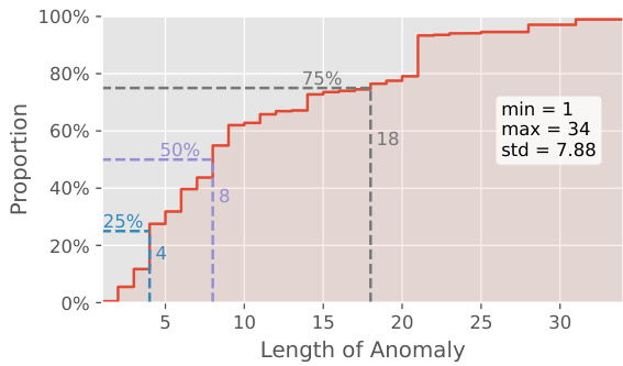
The figure shows the empirical cumulative distribution function of the lengths of anomalies for four datasets (SMD, PSM, SWaT, and HAI). It illustrates the distribution of anomaly durations, highlighting that some datasets exhibit shorter anomalies (SMD, PSM) while others show longer anomalies (SWaT, HAI). This visualization provides insights into the characteristics of anomalies in each dataset, informing the design and evaluation of anomaly detection methods.

This figure shows how the transformer model in SARAD captures spatial associations in a service monitoring benchmark. It visualizes the raw time series data, association matrices before, during, and after an anomaly, and the changes in associations (reductions) due to the anomaly. The anomalous features are highlighted, and it demonstrates the association reduction phenomenon (SAR) where anomalies cause a decrease in associations, particularly column-wise.
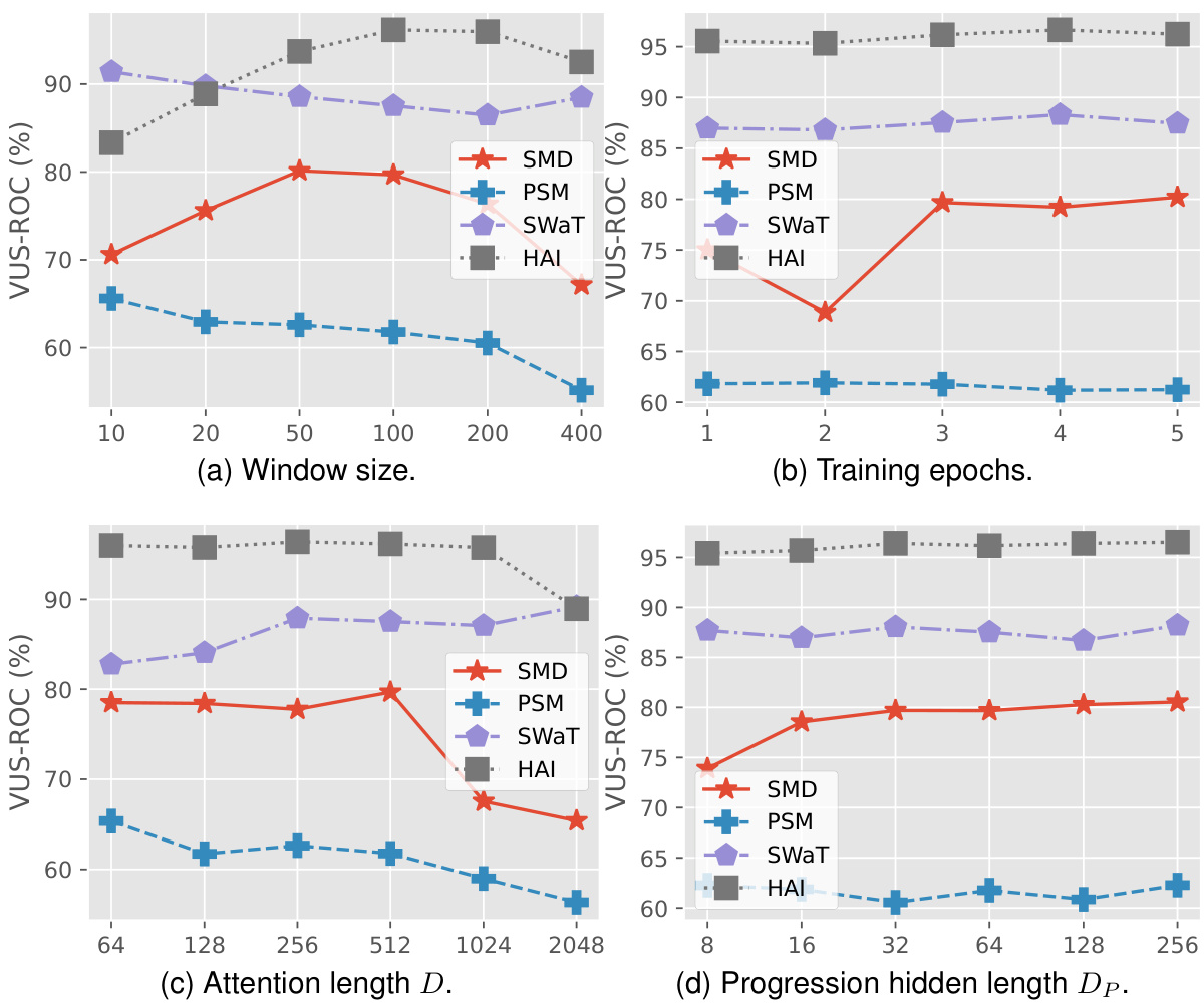
This figure shows how the transformer model in SARAD captures spatial associations in a service monitoring benchmark. It displays the raw time series data before, during, and after an anomaly, along with the association mappings (A) generated by the model at each stage. The darker the cell in the association mapping, the stronger the association between the corresponding features. The figure highlights how anomalous features exhibit a decrease in associations during the anomaly, particularly in the columns of the matrix. This phenomenon is described as Spatial Association Reduction (SAR) in the paper.

This figure shows how a transformer model captures spatial associations in a multivariate time series, specifically focusing on the changes in these associations before, during, and after an anomaly. The visualization uses heatmaps to represent the associations, with darker colors indicating stronger relationships. The figure highlights that anomalies cause a reduction in associations involving anomalous features, primarily in the columns of the association matrices.

This figure shows how the transformer model captures spatial associations between features in a multivariate time series, specifically focusing on changes in these associations before, during, and after an anomaly. The raw time series data is displayed alongside heatmaps representing the strength of associations between features. The heatmaps visually demonstrate a reduction in associations involving anomalous features during the anomaly, supporting the paper’s claim that anomalies disrupt spatial relationships.
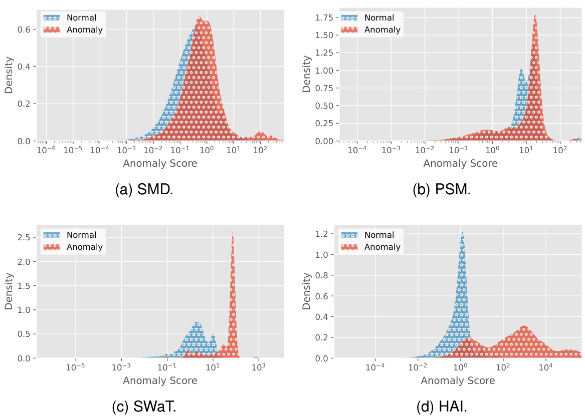
This figure shows how the transformer model captures spatial associations in a service monitoring benchmark. It highlights the changes in associations before, during, and after an anomaly. The key observation is that anomalies cause a reduction in associations, particularly among anomalous features. This reduction is visualized using heatmaps and difference maps.
More on tables

This table presents the statistics of four real-world datasets used in the paper’s experiments: Server Machine Dataset (SMD), Pooled Server Metrics (PSM), Secure Water Treatment (SWaT), and Hardware-In-the-Loop-based Augmented ICS (HAI). For each dataset, it lists the number of features, the size of the training set, the size of the test set, the number of anomalies, the ratio of anomalies, and the minimum, median, and maximum lengths of the anomalies. It also specifies the sampling period used for each dataset.

This table presents the anomaly detection performance using various metrics. It compares the performance of the proposed SARAD model against several other state-of-the-art methods across four different datasets (SMD, PSM, SWAT, HAI). The metrics used include AUC-ROC, AUC-PR, VUS-ROC, and VUS-PR. These metrics are calculated using five different random seeds, and the best and second-best performing methods are highlighted.

This table presents the anomaly diagnosis performance of different methods on four real-world datasets. It uses three common metrics: Hit Rate (HR@P%), Normalized Discounted Cumulative Gain (NDCG@P%), and Interpretation Score (IPS@P%). These metrics assess the accuracy of identifying anomalous features at both the point-wise and range-wise levels, considering various percentages (P%) of the top-ranked anomalous features. The results are averaged across five random seeds to provide a robust performance comparison.

This table presents the ablation study on the progression reconstruction module of SARAD. It shows the performance of SARAD under various changes made to the progression reconstruction submodules, including removing the ReLU activation function, using row sum instead of column sum for aggregation, fully concatenating the association mappings without any aggregation, and using the progression directly for detection instead of autoencoding it. The results highlight the importance of each submodule and the chosen design choices in achieving state-of-the-art performance.

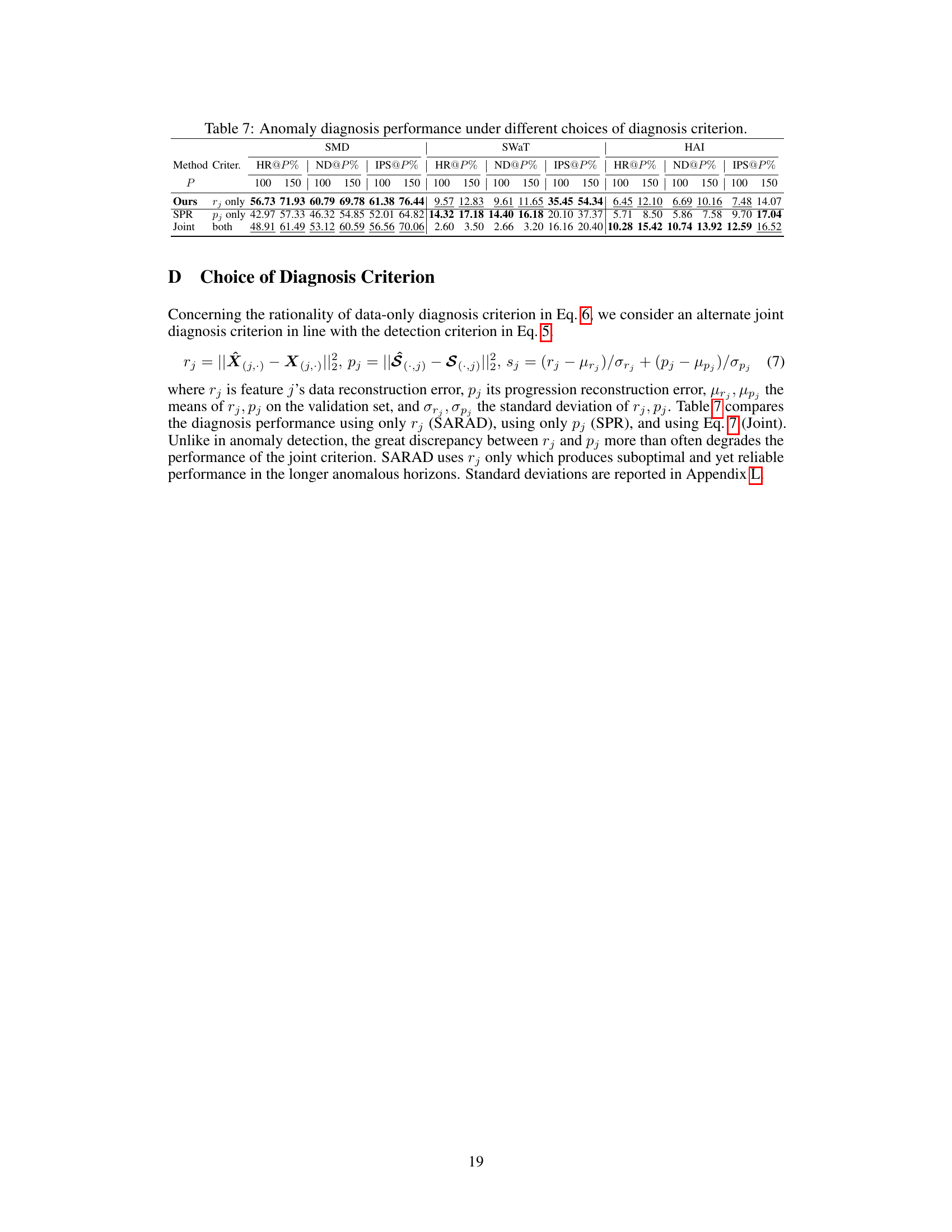
This table presents a comparison of anomaly detection performance using different criteria. The criteria compared are using only the data reconstruction error (DR), only the progression reconstruction error (SPR), and a joint criterion combining both (Joint). The performance is evaluated using Area Under the ROC Curve (AROC), Area Under the Precision-Recall Curve (APR), Volume Under the ROC Surface (VROC), and Volume Under the Precision-Recall Surface (VPR). The results are shown for four different datasets: SMD, PSM, SWAT, and HAI. This allows for assessing the relative contributions of the data and association-based components to the overall anomaly detection performance.

This table presents the anomaly diagnosis performance using three metrics: Hit Rate (HR@P%), Normalized Discounted Cumulative Gain (NDCG@P%), and Interpretation Score (IPS@P%). These metrics evaluate the accuracy of identifying the anomalous features at each time point. The results are averaged across five random seeds to account for variability and provide more reliable results. The P% values indicate different thresholds for the top-k ranked features.
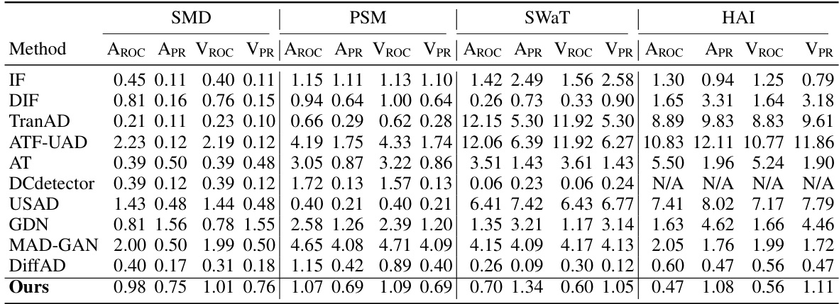
This table presents the anomaly detection performance of SARAD and several other state-of-the-art methods on four real-world datasets. The metrics used are threshold-independent AUC-ROC, AUC-PR, VUS-ROC, and VUS-PR. Higher values indicate better performance. The table highlights SARAD’s superior performance compared to other methods, particularly on the VUS-ROC metric. This suggests the robustness and generalizability of SARAD’s approach, especially considering that the VUS metrics are fully parameter-free and less susceptible to thresholding biases common in other evaluation methods.

This table presents the results of ablation studies on the progression reconstruction module of the SARAD model. It shows the Area Under the ROC Curve (AUC-ROC) and Area Under the Precision-Recall Curve (AUC-PR) scores, as well as the Volume Under the Surface (VUS) AUC-ROC and VUS-AUC-PR scores, for different variations of the progression reconstruction module. The variations include removing the ReLU activation function, changing the aggregation method from column sum to row sum, removing the aggregation step entirely, and using the progression directly for detection instead of reconstruction errors. The results show that the original design of the progression reconstruction module performs best in terms of anomaly detection performance.

This table presents the standard deviations of the anomaly detection performance metrics reported in Table 3 of the paper. The metrics include the threshold-independent Area Under the Curve for the Receiver Operating Characteristic (AUC-ROC) and the AUC for Precision-Recall curves (AUC-PR), as well as the fully parameter-free Volume Under the Surface for AUC-ROC (VUS-ROC) and AUC-PR (VUS-PR). The standard deviations are calculated from five random seeds, providing a measure of the variability in the results.

This table presents the anomaly diagnosis performance using three different metrics: Hit Rate (HR@P%), Normalized Discounted Cumulative Gain (NDCG@P%), and Interpretation Score (IPS@P%). Each metric is evaluated at different percentage levels (P) to measure the effectiveness of anomaly diagnosis. The results are averaged over five separate runs with different random seeds, providing a measure of the stability of the performance.

This table presents the anomaly diagnosis performance of different methods. It uses three common metrics: Hit Rate (HR@P%), Normalized Discounted Cumulative Gain (NDCG@P%), and Interpretation Score (IPS@P%). The metrics are calculated at different percentage thresholds (P%). The results are averaged across five different random seeds to account for variability.

This table presents the anomaly detection performance results of various methods on four different datasets (SMD, PSM, SWAT, HAI). The performance is evaluated using four metrics: Area Under the ROC Curve (AUC-ROC), Area Under the Precision-Recall Curve (AUC-PR), Volume Under the Surface AUC-ROC (VUS-ROC), and Volume Under the Surface AUC-PR (VUS-PR). The best performance for each metric on each dataset is shown in bold, and the second-best is underlined. The results are averaged over five different random seeds.

This table presents the anomaly detection performance of SARAD and other state-of-the-art methods. The performance is measured using four metrics: AUC-ROC, AUC-PR, VUS-ROC, and VUS-PR. Each metric is calculated across five different random seeds, and the best and second-best results are highlighted. The table is broken down by dataset and method, facilitating a comparison of different approaches on various real-world datasets.
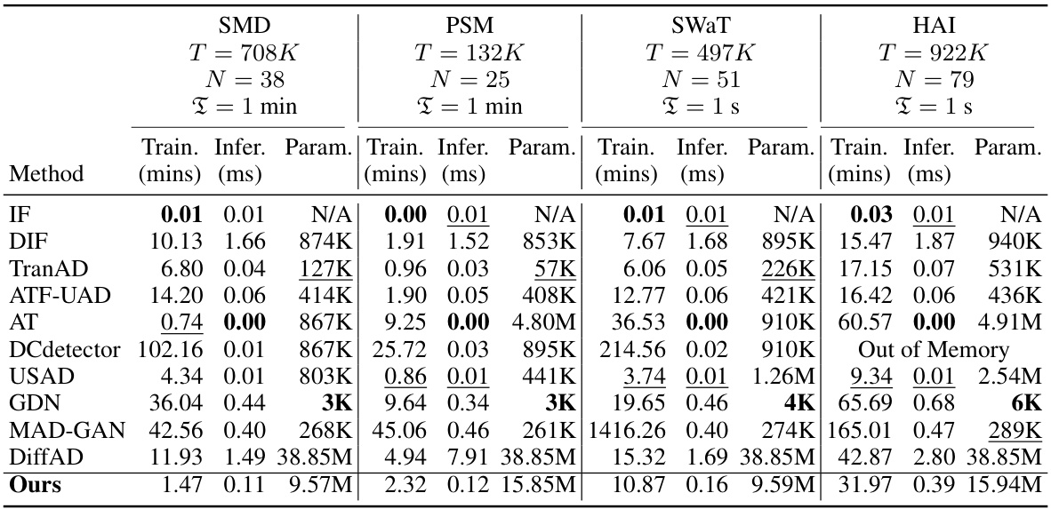
This table presents the training time, inference time per sample, and the number of parameters of different anomaly detection methods on four different datasets (SMD, PSM, SWAT, and HAI). The datasets vary in size, number of features, and sampling frequency, which impacts the training and inference time of each method. The table allows for comparing the efficiency and complexity of each method in terms of computational resources and speed.

This table presents the anomaly detection performance of SARAD and other state-of-the-art methods on four real-world datasets. The performance is measured using four metrics: AUC-ROC, AUC-PR, VUS-ROC, and VUS-PR. AUC-ROC and AUC-PR are threshold-independent, while VUS-ROC and VUS-PR are fully parameter-free. The table shows the average performance across five random seeds, with the best and second-best results highlighted.

This table presents the anomaly detection performance of SARAD and other state-of-the-art methods on four datasets. The performance is measured using four metrics: AUC-ROC, AUC-PR, VUS-ROC, and VUS-PR. AUC-ROC and AUC-PR are threshold-independent, while VUS-ROC and VUS-PR are fully parameter-free. The best and second-best results for each dataset are highlighted.
Full paper#
