TL;DR#
Current robust fine-tuning methods for vision-language models often neglect confidence calibration, leading to unreliable model outputs in out-of-distribution (OOD) scenarios. This paper tackles this issue by proposing a novel approach called CaRot. Existing methods improve OOD accuracy but often miscalibrate confidence, making it hard to trust model predictions.
CaRot simultaneously improves both OOD accuracy and confidence calibration by leveraging a theoretical insight that connects OOD classification and calibration errors to ID data characteristics. The proposed method combines a constrained multimodal contrastive loss and self-distillation to enhance the model’s robustness and calibration performance. Experimental results demonstrate its effectiveness compared to existing approaches on various ImageNet distribution shift benchmarks.
Key Takeaways#
Why does it matter?#
This paper is crucial for researchers working on robust fine-tuning of vision-language models. It addresses the critical issue of confidence calibration in OOD generalization, a significant limitation of current methods. By providing a novel framework and theoretical analysis, it significantly advances the field, opening new avenues for building more reliable and trustworthy AI systems. The theoretical findings offer a new perspective for future work on improving the robustness of foundation models and practical implementations offer valuable insights for other multimodal models.
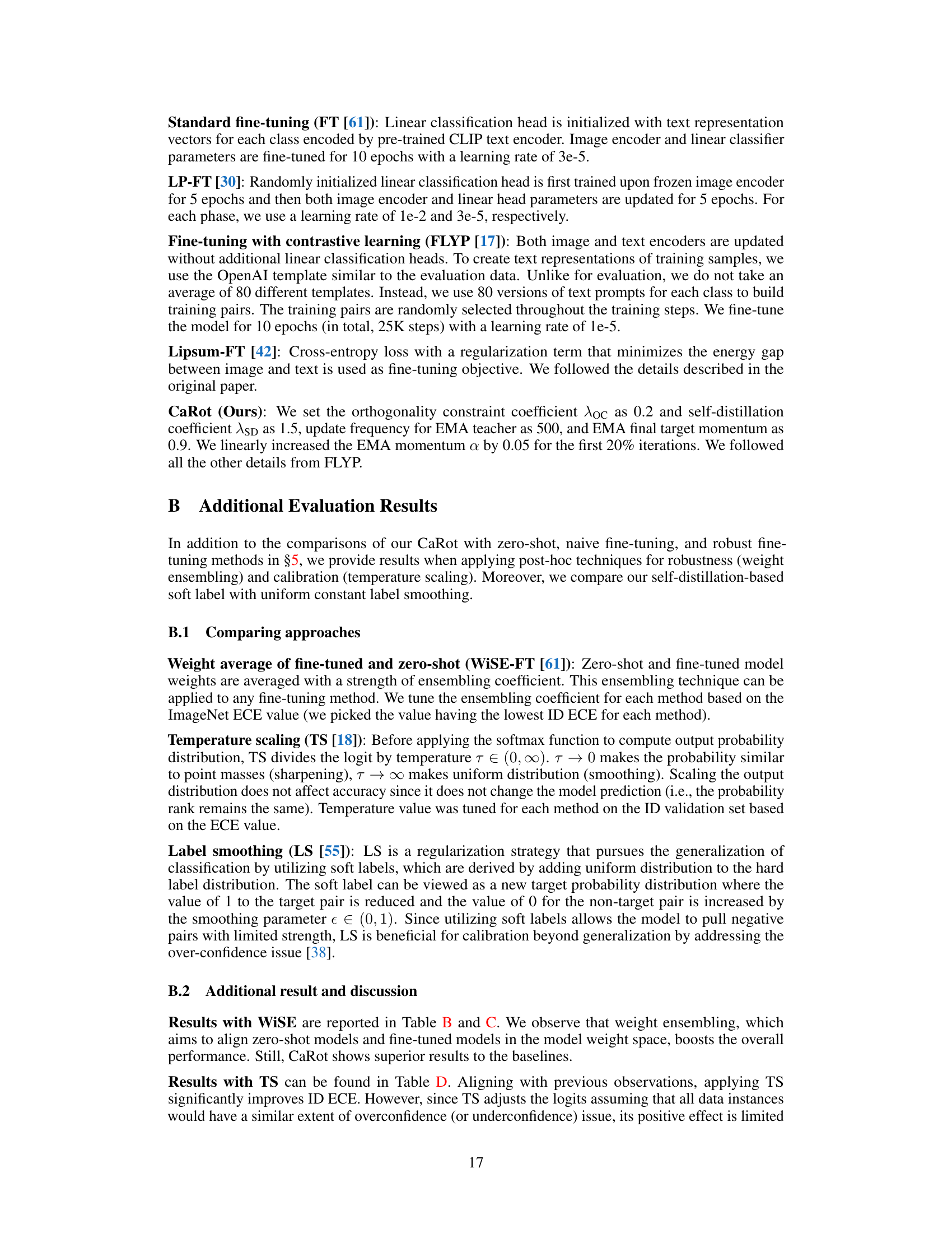
Visual Insights#
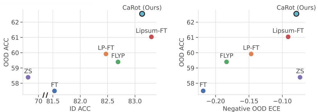
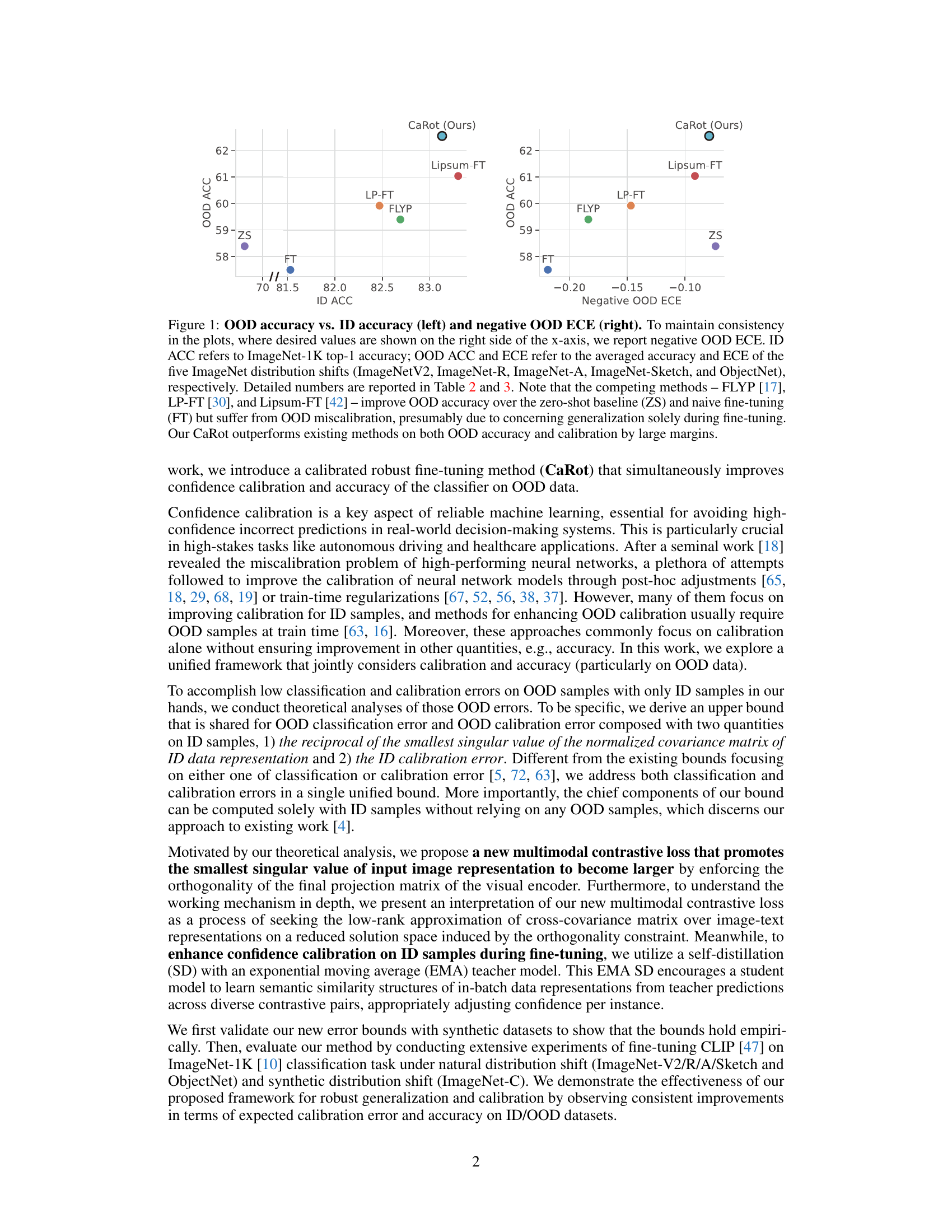
🔼 This figure compares various fine-tuning methods (FLYP, LP-FT, Lipsum-FT, and the proposed CaRot) against zero-shot (ZS) and standard fine-tuning (FT) baselines. The left panel shows OOD accuracy plotted against ID accuracy. The right panel shows negative OOD expected calibration error (ECE). The results demonstrate that while existing methods improve OOD accuracy, they suffer from poor calibration. In contrast, CaRot achieves superior performance in both OOD accuracy and calibration.
read the caption
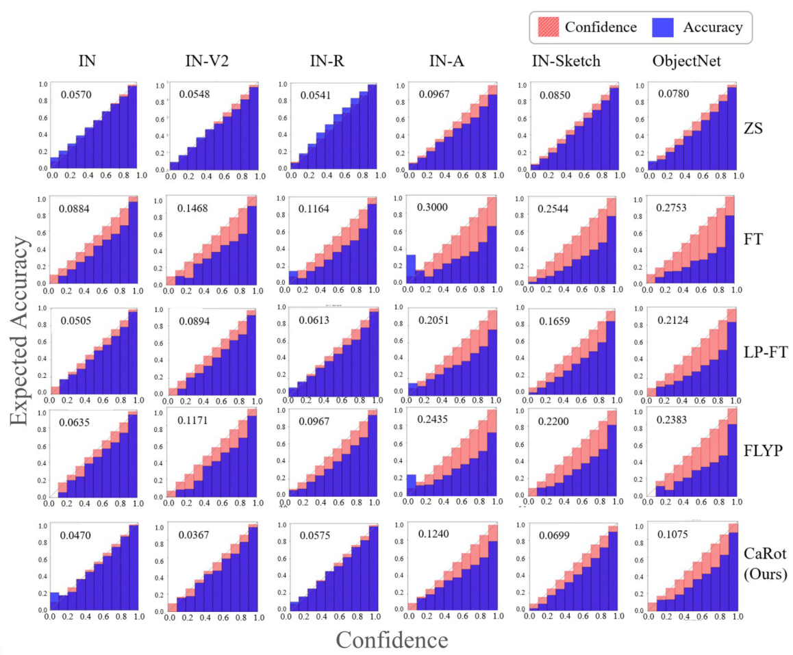
Figure 1: OOD accuracy vs. ID accuracy (left) and negative OOD ECE (right). To maintain consistency in the plots, where desired values are shown on the right side of the x-axis, we report negative OOD ECE. ID ACC refers to ImageNet-1K top-1 accuracy; OOD ACC and ECE refer to the averaged accuracy and ECE of the five ImageNet distribution shifts (ImageNetV2, ImageNet-R, ImageNet-A, ImageNet-Sketch, and ObjectNet), respectively. Detailed numbers are reported in Table 2 and 3. Note that the competing methods – FLYP [17], LP-FT [30], and Lipsum-FT [42] – improve OOD accuracy over the zero-shot baseline (ZS) and naive fine-tuning (FT) but suffer from OOD miscalibration, presumably due to concerning generalization solely during fine-tuning. Our CaRot outperforms existing methods on both OOD accuracy and calibration by large margins.

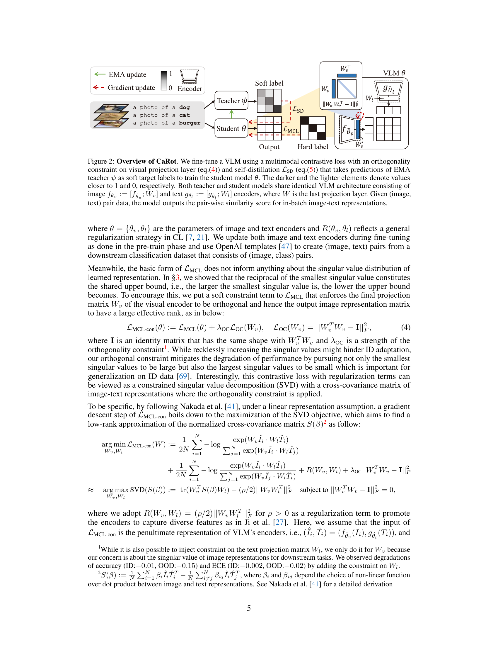
🔼 This table presents the best values obtained for the two components of the RHS (right-hand side) of the inequality derived in Theorem 3 of the paper: the ID calibration error (ECE) and the reciprocal of the smallest singular value of the ID input covariance matrix (σmin). It also displays the corresponding LHS (left-hand side) values representing the OOD (out-of-distribution) errors in terms of Mean Squared Error (MSE) and Expected Calibration Error (ECE). The results showcase the improvements in OOD performance by reducing the upper bound as defined in the theorem. Note that higher σmin and lower ECE values are desirable. The results are averages over three repetitions of the experiments.
read the caption
Table 1: The best case values of two terms of RHS (ID Omin and ID ECE) and LHS – OOD errors (MSE and ECE) in the bounds of Theorem 3. Reported values are an average of three repeated runs.
In-depth insights#
OOD Calibration#
Out-of-distribution (OOD) calibration is a crucial aspect of robust machine learning, especially for high-stakes applications. Improper calibration leads to unreliable model confidence scores, hindering trust and decision-making. Existing robust fine-tuning methods often prioritize OOD accuracy over calibration, resulting in high-confidence, incorrect predictions. A well-calibrated model should ideally exhibit confidence scores that accurately reflect the model’s true predictive accuracy across both in-distribution (ID) and OOD settings. Theoretical analysis of OOD calibration error often involves upper bounds that highlight factors like ID calibration error and the smallest singular value of the ID input covariance matrix. Effective OOD calibration strategies should aim to reduce these upper bounds, improving the reliability of model outputs. Techniques like self-distillation and constrained multimodal contrastive learning have shown promise in achieving this goal, but further research is needed to fully understand the mechanisms and address challenges in the context of real-world deployment.
Contrastive Loss#
Contrastive loss, a crucial component in many deep learning models, particularly excels in self-supervised learning scenarios. By encouraging similar data points to cluster together while separating dissimilar ones in an embedding space, it learns robust representations. This approach is particularly powerful for vision-language models, where it facilitates learning joint representations that capture the semantic relationships between images and their textual descriptions. The effectiveness of contrastive loss is heavily influenced by several factors such as the choice of architecture, the definition of similarity, and the temperature parameter. Furthermore, the computational demands of contrastive loss, especially with large datasets, are significant, and the effectiveness of various contrastive loss functions can vary greatly depending on the specific task. Optimization strategies and techniques to address computational bottlenecks are essential for maximizing the benefits of contrastive learning.
Theoretical Bounds#
A section on theoretical bounds in a research paper would ideally present a rigorous mathematical framework to quantify the performance limits of a given model or algorithm. Key aspects would include clearly stated assumptions, precise definitions of relevant metrics, and a step-by-step derivation of the bounds themselves. The discussion should emphasize the significance of the bounds in practice, highlighting their implications for model design, training, and deployment. Ideally, comparisons to existing bounds would be provided, analyzing the advantages and disadvantages of the new bounds. A thorough analysis would consider both the strengths and limitations of the theoretical results, acknowledging any simplifying assumptions made during the derivation and discussing how these might affect the practical applicability of the findings. The paper should also address the tightness of the bounds: how close are the theoretical limits to the actual observed performance? Finally, the theoretical analysis should motivate practical insights for improving the model or algorithm’s performance, possibly guiding the design of improved algorithms or suggesting new research directions.
Empirical Results#
The Empirical Results section of a research paper is crucial for validating the claims and hypotheses presented. A strong section will thoroughly detail experiments designed to test the proposed methods, showing not only performance metrics but also the experimental setup, data sources, and the rationale behind the chosen evaluation measures. Statistical significance should be clearly reported, along with error bars or confidence intervals, and the results should be discussed in the context of prior work and limitations. Clear visualization of results through charts and graphs is also critical to easily convey trends and patterns in the data, enabling the reader to quickly grasp the main findings. Robustness testing under various conditions, such as changes in parameters or data distributions, would further strengthen the reported empirical results and enhance their credibility and significance. The discussion should also highlight any unexpected or counter-intuitive outcomes, and the limitations of the experiments should be openly acknowledged. A comprehensive empirical results section ultimately provides the strongest evidence of a study’s validity and impact.
Future Work#
Future research directions stemming from this work could explore several promising avenues. Extending the theoretical framework to encompass a broader range of model architectures and tasks beyond CLIP’s image classification is crucial. Investigating the impact of different regularization techniques and their interplay with the proposed multimodal contrastive loss would provide a deeper understanding. Empirically validating the theoretical bounds on more diverse and challenging distribution shift benchmarks beyond the ImageNet variations is necessary to establish generalizability. Furthermore, a comprehensive analysis of the trade-offs between ID and OOD performance, calibration, and computational cost should be conducted, leading to more practical guidelines for robust fine-tuning. Finally, exploring the application of this framework to other modalities (e.g., text, audio) and investigating its potential for mitigating biases in foundation models would be highly beneficial.
More visual insights#
More on figures

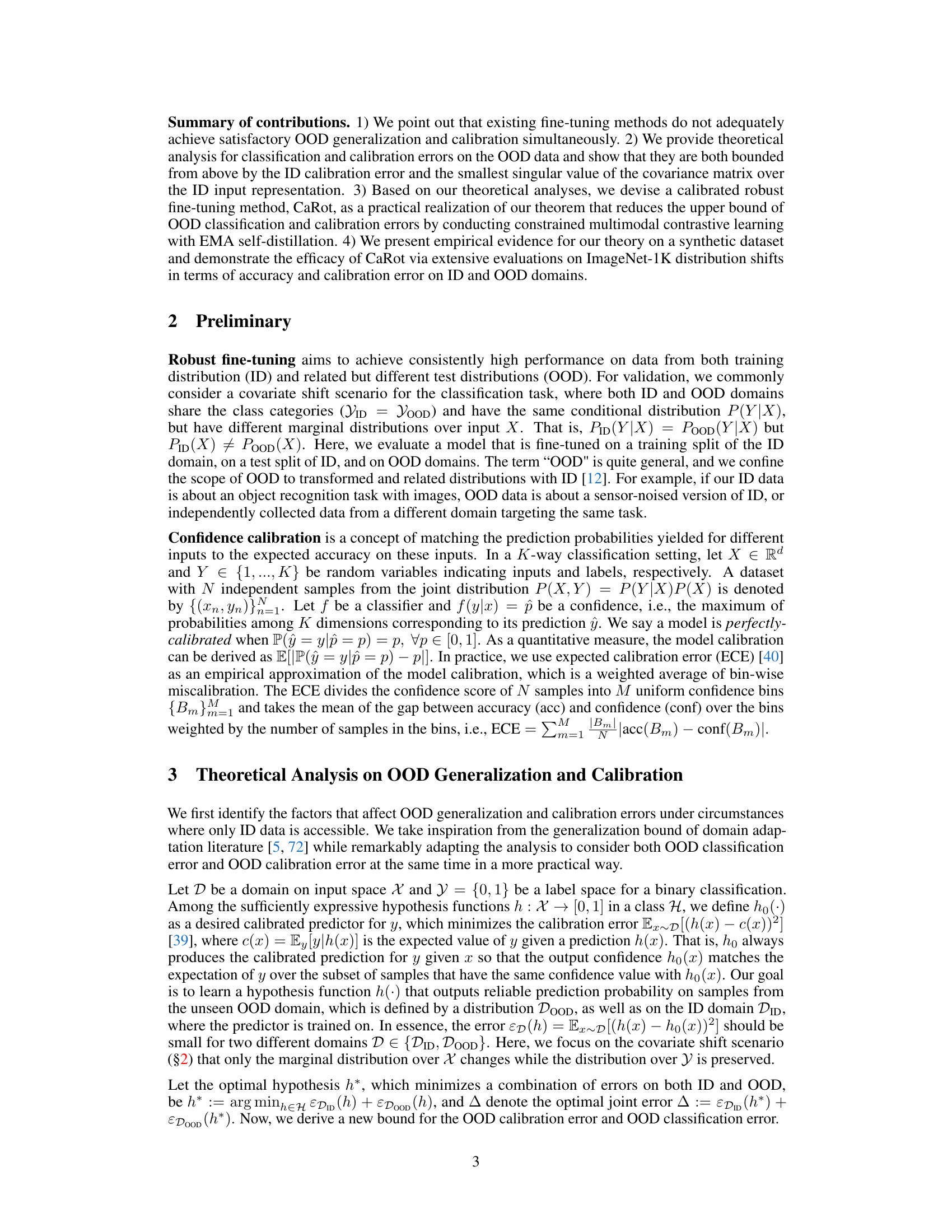
🔼 This figure illustrates the proposed CaRot framework, which fine-tunes a Vision-Language Model (VLM) using a novel multimodal contrastive loss with an orthogonality constraint and self-distillation. The diagram shows the interaction between the student and teacher models, emphasizing the use of soft labels derived from the teacher’s predictions for self-distillation, and a constraint on the visual projection matrix. The overall process aims to enhance confidence calibration and accuracy by increasing the smallest singular value of the ID input covariance matrix while improving ID calibration.
read the caption
Figure 2: Overview of CaRot. We fine-tune a VLM using a multimodal contrastive loss with an orthogonality constraint on visual projection layer (eq.(4)) and self-distillation LSD (eq.(5)) that takes predictions of EMA teacher ψ as soft target labels to train the student model θ. The darker and the lighter elements denote values closer to 1 and 0, respectively. Both teacher and student models share identical VLM architecture consisting of image fθv := [fθ̂; Wv] and text gθt := [gθ̂₁; Wt] encoders, where W is the last projection layer. Given (image, text) pair data, the model outputs the pair-wise similarity score for in-batch image-text representations.

🔼 This figure empirically validates the theoretical error bounds presented in section 3 of the paper. The left plot shows the relationship between the right-hand side (RHS) of inequality (2) (OOD MSE) and the average of the reciprocal of the minimum singular value of the ID data’s covariance matrix and the ID ECE. The right plot shows the same for inequality (1) (OOD ECE). The strong negative correlation supports the theory that minimizing the RHS can reduce the OOD errors. The plots show that reducing ID calibration error and increasing the minimum singular value of the ID input covariance matrix (which is a measure of the diversity of the input features) results in lower OOD classification and calibration errors.
read the caption
Figure 3: Analysis of error bounds on synthetic data. Plots on the left side show RHS (x-axis) and LHS (y-axis; MSE for ineq.(2) and ECE for ineq.(1)) of the inequalities in §3. We denote MSE for the mean squared error, Loc for the singular value regularization, and LSD for the calibration regularization.
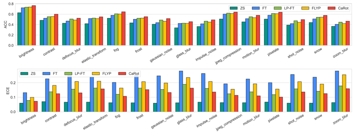
🔼 This figure shows the performance comparison of different fine-tuning methods (ZS, FT, LP-FT, FLYP, CaRot) on ImageNet-C dataset. ImageNet-C is a corrupted version of ImageNet dataset with 15 types of corruptions and 5 severity levels. The top part shows the accuracy for each corruption type, while the bottom shows the Expected Calibration Error (ECE). The results demonstrate that CaRot consistently outperforms other methods across various corruptions.
read the caption
Figure 4: IN-C corruption-wise accuracy (top) and ECE (bottom). We evaluate accuracy and ECE over 15 types of image corruption with five corruption severity and report the average performance per corruption. CaRot consistently outperforms baseline methods across diverse corruptions.

🔼 This figure shows box plots of accuracy for different fine-tuning methods (ZS, FT, LP-FT, FLYP, CaRot) on two specific corruptions from the ImageNet-C dataset: brightness and elastic_transform. It highlights that CaRot’s performance improvement over baselines is more pronounced for coarser corruptions (brightness) compared to finer-grained corruptions (elastic_transform).
read the caption
Figure 5: Closer look at the effectiveness of CaRot on different corruptions. We provide IN-C accuracy on brightness (left) and elastic transform (right) corruptions. CaRot excels on the coarser corruption such as brightness whereas its effectiveness is weakened on the finer corruption such as elastic transform.

🔼 This figure shows the impact of using the constrained multi-modal contrastive loss (LMCL-con) on the smallest 20 singular values of the image representation covariance matrix. The LMCL-con loss increases these singular values compared to the unconstrained LMCL loss, which supports the theoretical finding that increasing the smallest singular value helps to improve out-of-distribution generalization.
read the caption
Figure 6: Impact of LMCL-con. Analysis on singular values. Figure 6 illustrates the last 20 singular values of the covariance matrix \(\mathbf{I}^T \mathbf{I}\) where \(\mathbf{I}\) is a standardized image representations over \(N\) samples. Our proposed constrained contrastive loss \(\mathcal{L}_{\text{MCL-con}}\) increases the small singular values compared to the vanilla contrastive loss \(\mathcal{L}_{\text{MCL}}\). This result verifies that adding the orthogonality constraint successfully reduces \(1/\sigma_{\text{min}}(\mathbf{D}_{\text{ID}})\), the component of the shared upper bound we derived in §3, following our intention.
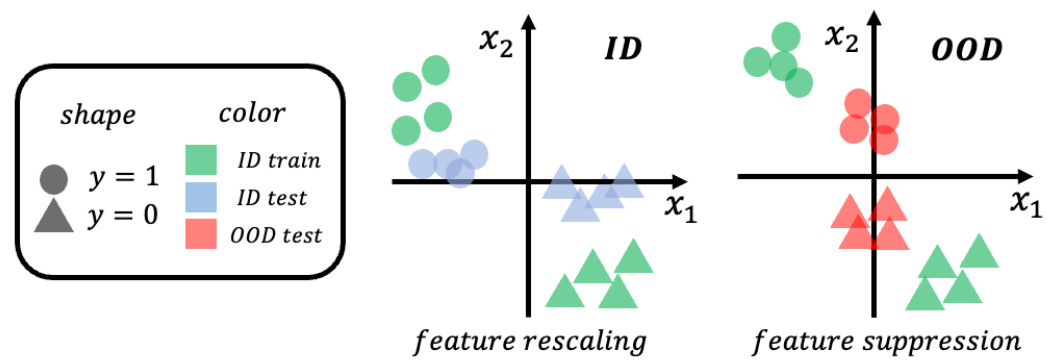
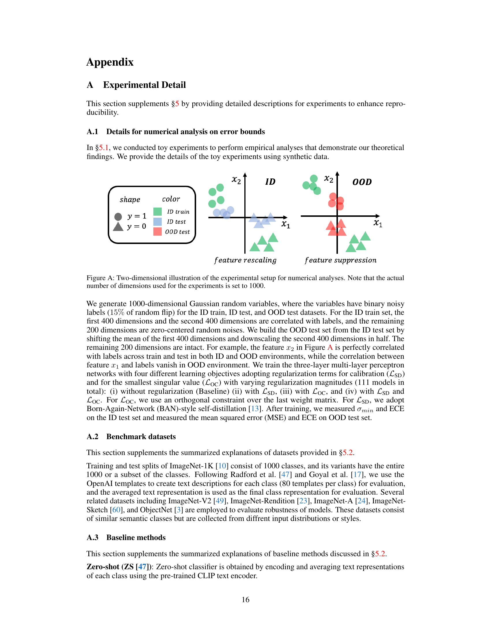
🔼 This figure is a 2D illustration of how the synthetic datasets are created for the numerical analysis in section 5.1. The ID datasets have two features (x1 and x2) correlated with the labels, while OOD data is generated by manipulating these features to simulate a shift in distribution. Specifically, for x1, the mean is shifted, and for x2, the scale is reduced in the OOD data. The figure helps visualize the covariate shift involved in the experiments.
read the caption
Figure A. Two-dimensional illustration of the experimental setup for numerical analyses. Note that the actual number of dimensions used for the experiments is set to 1000.
🔼 The figure compares different robust fine-tuning methods on their out-of-distribution (OOD) accuracy and expected calibration error (ECE). It shows that while some methods improve OOD accuracy, they often suffer from poor calibration. The proposed method, CaRot, achieves both high OOD accuracy and good calibration.
read the caption
Figure 1: OOD accuracy vs. ID accuracy (left) and negative OOD ECE (right). To maintain consistency in the plots, where desired values are shown on the right side of the x-axis, we report negative OOD ECE. ID ACC refers to ImageNet-1K top-1 accuracy; OOD ACC and ECE refer to the averaged accuracy and ECE of the five ImageNet distribution shifts (ImageNetV2, ImageNet-R, ImageNet-A, ImageNet-Sketch, and ObjectNet), respectively. Detailed numbers are reported in Table 2 and 3. Note that the competing methods – FLYP [17], LP-FT [30], and Lipsum-FT [42] – improve OOD accuracy over the zero-shot baseline (ZS) and naive fine-tuning (FT) but suffer from OOD miscalibration, presumably due to concerning generalization solely during fine-tuning. Our CaRot outperforms existing methods on both OOD accuracy and calibration by large margins.
More on tables

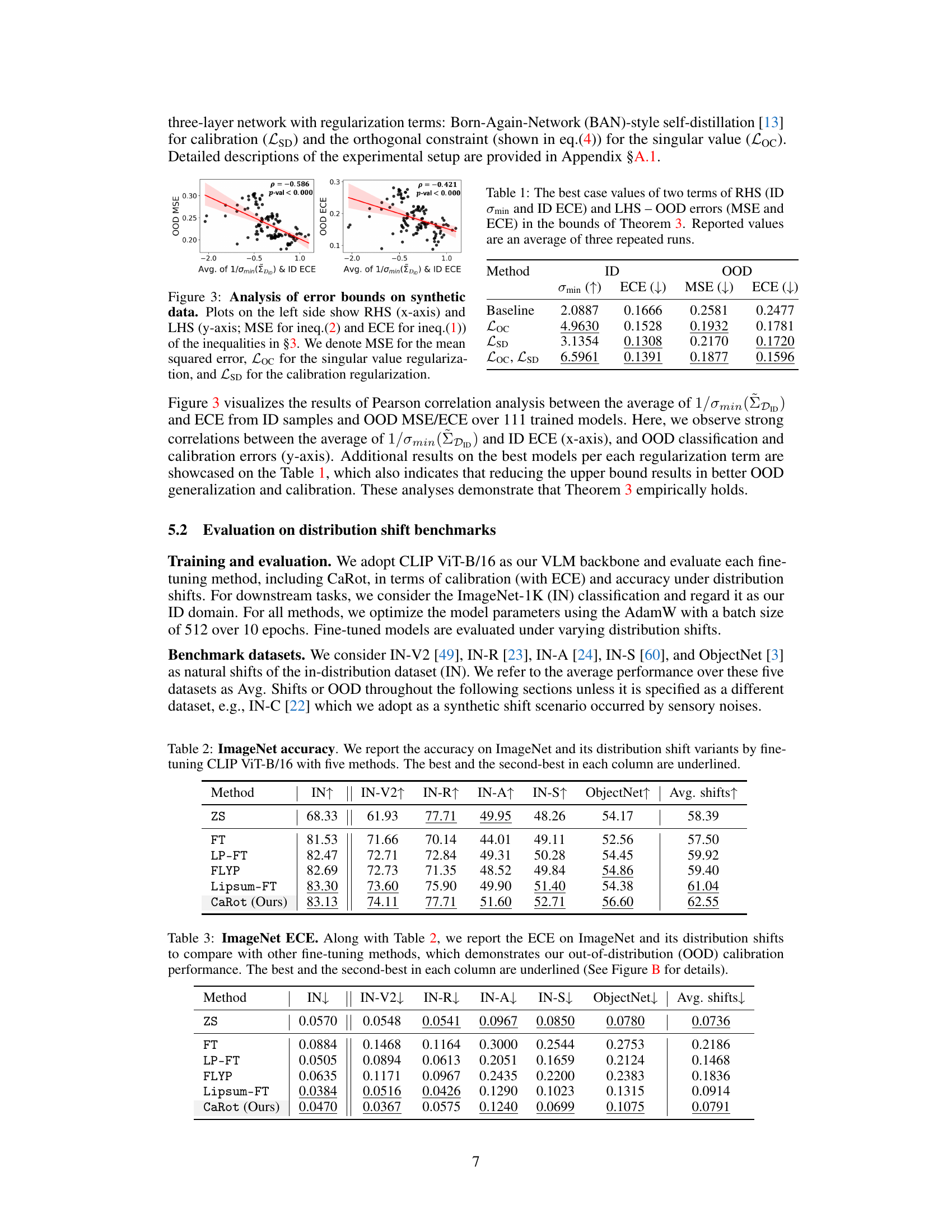
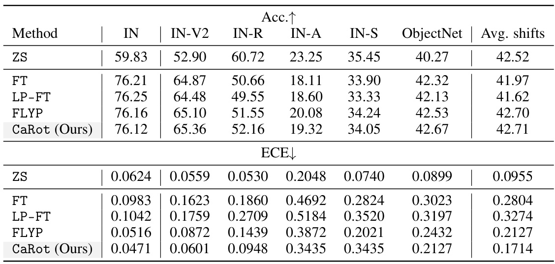
🔼 This table shows the accuracy results on ImageNet and five of its distribution shift variants (ImageNetV2, ImageNet-R, ImageNet-A, ImageNet-Sketch, and ObjectNet). The accuracy is reported for five different fine-tuning methods: Zero-Shot (ZS), standard Fine-Tuning (FT), LP-FT, FLYP, and Lipsum-FT. The best and second-best performing methods for each dataset are underlined.
read the caption
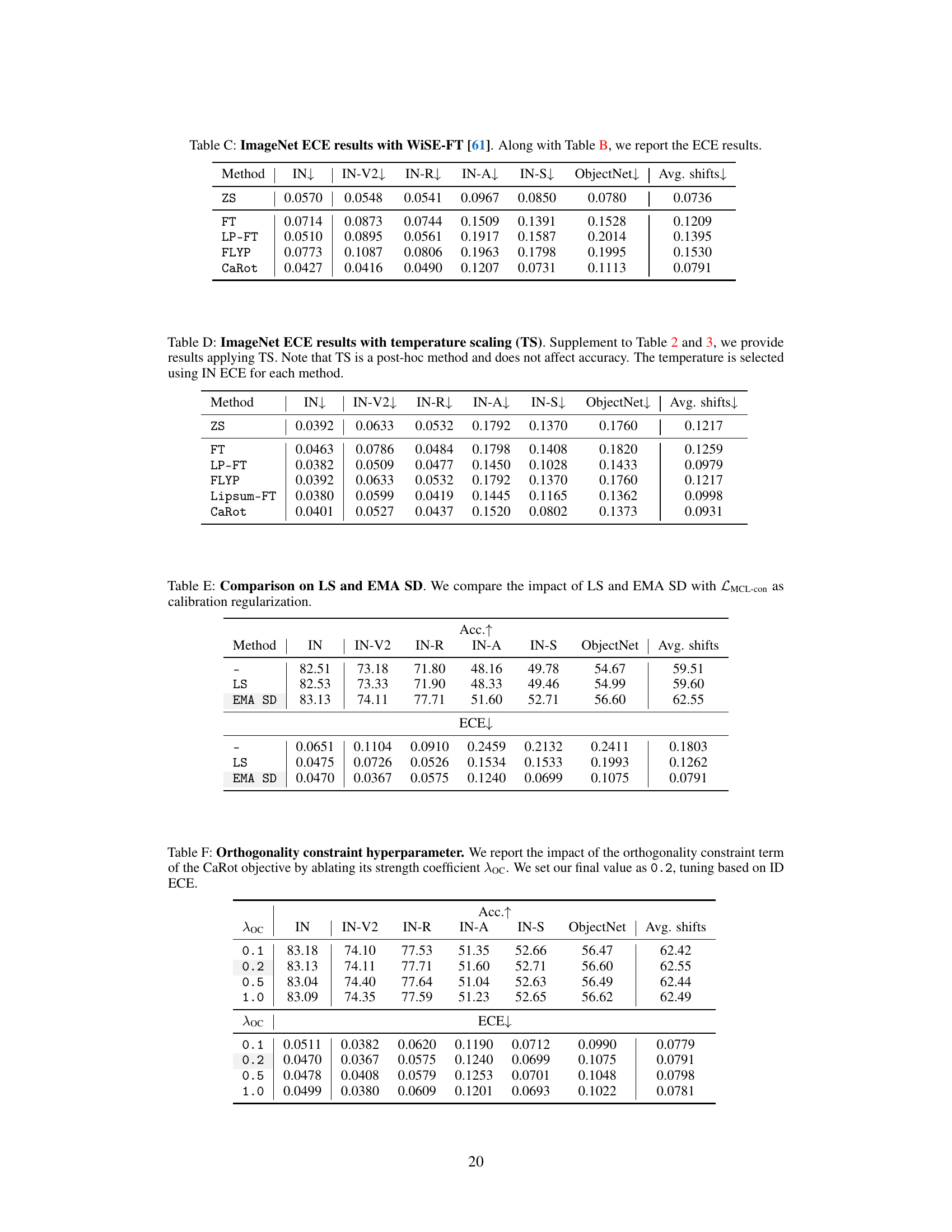
Table 2: ImageNet accuracy. We report the accuracy on ImageNet and its distribution shift variants by fine-tuning CLIP ViT-B/16 with five methods. The best and the second-best in each column are underlined.

🔼 This table compares different fine-tuning methods on their expected calibration error (ECE) across various ImageNet datasets (including the original ImageNet-1K and several out-of-distribution datasets). Lower ECE values indicate better calibration. The best and second-best performing methods are highlighted for each dataset.
read the caption
Table 3: ImageNet ECE. Along with Table 2, we report the ECE on ImageNet and its distribution shifts to compare with other fine-tuning methods, which demonstrates our out-of-distribution (OOD) calibration performance. The best and the second-best in each column are underlined (See Figure B for details).

🔼 This table presents the ablation study results for the CaRot model. It shows the impact of each component (LMCL, LOC, and LSD) on the model’s performance in terms of accuracy and expected calibration error (ECE) on both in-distribution (ImageNet) and out-of-distribution datasets. The results are presented to highlight the contribution of each component to the overall improvement in OOD generalization and calibration.
read the caption
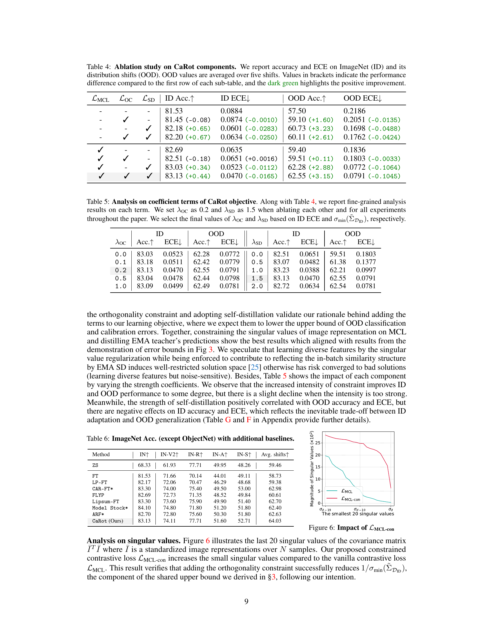
Table 4: Ablation study on CaRot components. We report accuracy and ECE on ImageNet (ID) and its distribution shifts (OOD). OOD values are averaged over five shifts. Values in brackets indicate the performance difference compared to the first row of each sub-table, and the dark green highlights the positive improvement.

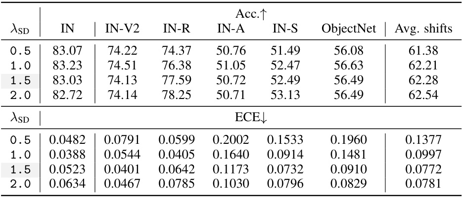
🔼 This table presents the ablation study results of the hyperparameters associated with the CaRot objective function. It shows how varying the strength coefficients λoc (for the orthogonality constraint) and λSD (for self-distillation) impact the performance in terms of accuracy (Acc.) and expected calibration error (ECE) on both the in-distribution (ID) and out-of-distribution (OOD) datasets. The final values of these hyperparameters (λoc = 0.2 and λSD = 1.5) were chosen based on the ID ECE and the minimum singular value of the ID data covariance matrix.
read the caption
Table 5. Analysis on coefficient terms of CaRot objective. Along with Table 4, we report fine-grained analysis results on each term. We set λoc as 0.2 and λSD as 1.5 when ablating each other and for all experiments throughout the paper. We select the final values of λoc and λSD based on ID ECE and σmin(DID), respectively.

🔼 This table presents the ImageNet classification accuracy results for various methods, including zero-shot (ZS), fine-tuning (FT), and several robust fine-tuning approaches (LP-FT, FLYP, Lipsum-FT, CAR-FT, Model Stock, ARF), and the proposed CaRot method. The accuracy is evaluated on the ImageNet dataset and its five distribution shift variants (IN-V2, IN-R, IN-A, IN-S, ObjectNet). The average accuracy across all six datasets is also reported. The table highlights CaRot’s superior performance compared to existing methods in achieving robust generalization under distribution shifts.
read the caption
Table 6: ImageNet Acc. (except ObjectNet) with additional baselines.

🔼 This table presents a summary of the ImageNet accuracy and ECE (Expected Calibration Error) results obtained using two different backbones: ResNet50 and ViT-L/14. It compares the performance of several fine-tuning methods (Zero-Shot, Fine-tuning, LP-FT, FLYP, and CaRot) across various metrics, highlighting the best and second-best results for each metric on both backbones.
read the caption
Table 7: ImageNet accuracy and ECE on different backbones. We provide summarized results on CLIP RN50 and ViT-L/14. The best and the second-best in each column are underlined. (See Table H and I for details.)

🔼 This table compares the performance of two different regularization techniques: SVD-based regularization and orthogonality constraint. Both methods aim to improve out-of-distribution (OOD) generalization and calibration. The table shows that while both methods achieve similar improvements, the SVD-based approach is computationally much more expensive. The comparison is made across several metrics, including accuracy and expected calibration error (ECE), for both in-distribution (ID) and OOD data. The ID-OOD Gap columns highlight the differences between ID and OOD performance.
read the caption
Table A: Comparison between SVD-based regularization and the orthogonality constraint term. Both terms are effective in terms of OOD generalization and calibration, but SVD requires a much heavier computation.

🔼 This table presents the ImageNet top-1 accuracy results for different fine-tuning methods across various distribution shift benchmarks. The methods compared are Zero-Shot (ZS), Fine-tuning (FT), LP-FT, FLYP, and the proposed CaRot method. The benchmarks include the original ImageNet dataset (IN) and five distribution shifts: IN-V2, IN-R, IN-A, IN-S, and ObjectNet. The table highlights the best and second-best performing methods for each benchmark, offering a clear comparison of the methods’ generalization capabilities under different distribution shifts.
read the caption
Table 2: ImageNet accuracy. We report the accuracy on ImageNet and its distribution shift variants by fine-tuning CLIP ViT-B/16 with five methods. The best and the second-best in each column are underlined.

🔼 This table compares the Expected Calibration Error (ECE) of different fine-tuning methods on ImageNet and five of its distribution shift variants (ImageNetV2, ImageNet-R, ImageNet-A, ImageNet-Sketch, and ObjectNet). Lower ECE values indicate better calibration, meaning the model’s confidence scores are closer to its actual accuracy. The table highlights the superior calibration performance of the proposed CaRot method, especially in out-of-distribution settings.
read the caption
Table 3: ImageNet ECE. Along with Table 2, we report the ECE on ImageNet and its distribution shifts to compare with other fine-tuning methods, which demonstrates our out-of-distribution (OOD) calibration performance. The best and the second-best in each column are underlined (See Figure B for details).

🔼 This table presents the Expected Calibration Error (ECE) for different fine-tuning methods on ImageNet and five of its distribution shift variants (ImageNetV2, ImageNet-R, ImageNet-A, ImageNet-Sketch, and ObjectNet). Lower ECE values indicate better calibration. The table allows a comparison of the calibration performance of the proposed method (CaRot) against existing state-of-the-art methods.
read the caption
Table 3: ImageNet ECE. Along with Table 2, we report the ECE on ImageNet and its distribution shifts to compare with other fine-tuning methods, which demonstrates our out-of-distribution (OOD) calibration performance. The best and the second-best in each column are underlined (See Figure B for details).

🔼 This table presents a fine-grained ablation study on the hyperparameters λloc and λSD of the CaRot objective function. It shows the impact of varying these parameters on the model’s performance in terms of accuracy and expected calibration error (ECE) on both in-distribution (ID) and out-of-distribution (OOD) datasets. The final values of λloc and λSD used in the main experiments were determined based on the ID ECE and the minimum singular value (σmin(DID)) of the ID data.
read the caption
Table 5: Analysis on coefficient terms of CaRot objective. Along with Table 4, we report fine-grained analysis results on each term. We set λloc as 0.2 and λSD as 1.5 when ablating each other and for all experiments throughout the paper. We select the final values of λloc and λSD based on ID ECE and σmin(DID), respectively.

🔼 This table presents the ablation study results for the CaRot model. It shows the impact of each component (LMCL, LOC, LSD) on the model’s performance in terms of accuracy and Expected Calibration Error (ECE) on both in-distribution (ID) ImageNet and out-of-distribution (OOD) datasets. The results demonstrate the contribution of each component to improving the overall performance.
read the caption
Table 4: Ablation study on CaRot components. We report accuracy and ECE on ImageNet (ID) and its distribution shifts (OOD). OOD values are averaged over five shifts. Values in brackets indicate the performance difference compared to the first row of each sub-table, and the dark green highlights the positive improvement.
🔼 This ablation study analyzes the impact of each component of the proposed CaRot model on ImageNet and five out-of-distribution (OOD) datasets. It shows the individual contributions of the constrained multimodal contrastive loss (LMCL-con), the orthogonality constraint (LOC), and the exponential moving average self-distillation (LSD). The table presents accuracy and expected calibration error (ECE) for both ID and OOD data, highlighting the positive effects of each component and their combined impact on model performance.
read the caption
Table 4: Ablation study on CaRot components. We report accuracy and ECE on ImageNet (ID) and its distribution shifts (OOD). OOD values are averaged over five shifts. Values in brackets indicate the performance difference compared to the first row of each sub-table, and the dark green highlights the positive improvement.
🔼 This table presents the ImageNet top-1 accuracy and average accuracy across five ImageNet distribution shift benchmarks (ImageNetV2, ImageNet-R, ImageNet-A, ImageNet-Sketch, and ObjectNet) for five different fine-tuning methods: zero-shot (ZS), standard fine-tuning (FT), LP-FT, FLYP, and Lipsum-FT. The best and second-best performing methods for each dataset are highlighted.
read the caption
Table 2: ImageNet accuracy. We report the accuracy on ImageNet and its distribution shift variants by fine-tuning CLIP ViT-B/16 with five methods. The best and the second-best in each column are underlined.
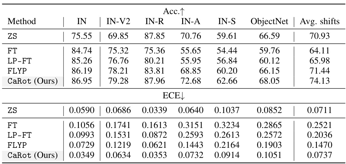
🔼 This table presents the ImageNet top-1 accuracy and average accuracy across five distribution shift benchmarks (ImageNetV2, ImageNet-R, ImageNet-A, ImageNet-Sketch, and ObjectNet) for five different methods: zero-shot (ZS), fine-tuning (FT), LP-FT, FLYP, and CaRot (the proposed method). The best performing method for each dataset is underlined.
read the caption
Table 2: ImageNet accuracy. We report the accuracy on ImageNet and its distribution shift variants by fine-tuning CLIP ViT-B/16 with five methods. The best and the second-best in each column are underlined.
Full paper#

