TL;DR#
Neural Ordinary Differential Equations (NODEs) offer an efficient way to model continuous-depth systems, but their training often involves computationally expensive numerical simulations. This paper tackles this issue by proposing a simulation-free training method for NODEs. The core idea is to directly regress the model’s dynamics to a predefined target velocity field, a technique called flow matching. However, applying flow matching directly to data pairs can lead to problematic crossing trajectories.
To address this, the authors cleverly employ flow matching in the embedding space of data pairs. They learn encoders that project data into this embedding space, jointly optimizing them with the dynamics function to ensure the validity and smoothness of the flow. This ensures that the learned dynamics correctly map input-output pairs. This approach outperforms previous NODE methods, especially in scenarios where the number of function evaluations is limited, by reducing computational costs and achieving higher accuracy in regression and classification tasks.
Key Takeaways#
Why does it matter?#
This paper is important because it significantly reduces the computational cost of training Neural Ordinary Differential Equations (NODEs) for deterministic tasks, a major challenge that has limited their broader application. The proposed method is highly relevant to current research trends in continuous-depth models and opens up new avenues for research in efficient and scalable NODEs training. Its practical implications extend to various applications where deterministic mapping between data is crucial, including but not limited to regression and classification tasks.
Visual Insights#

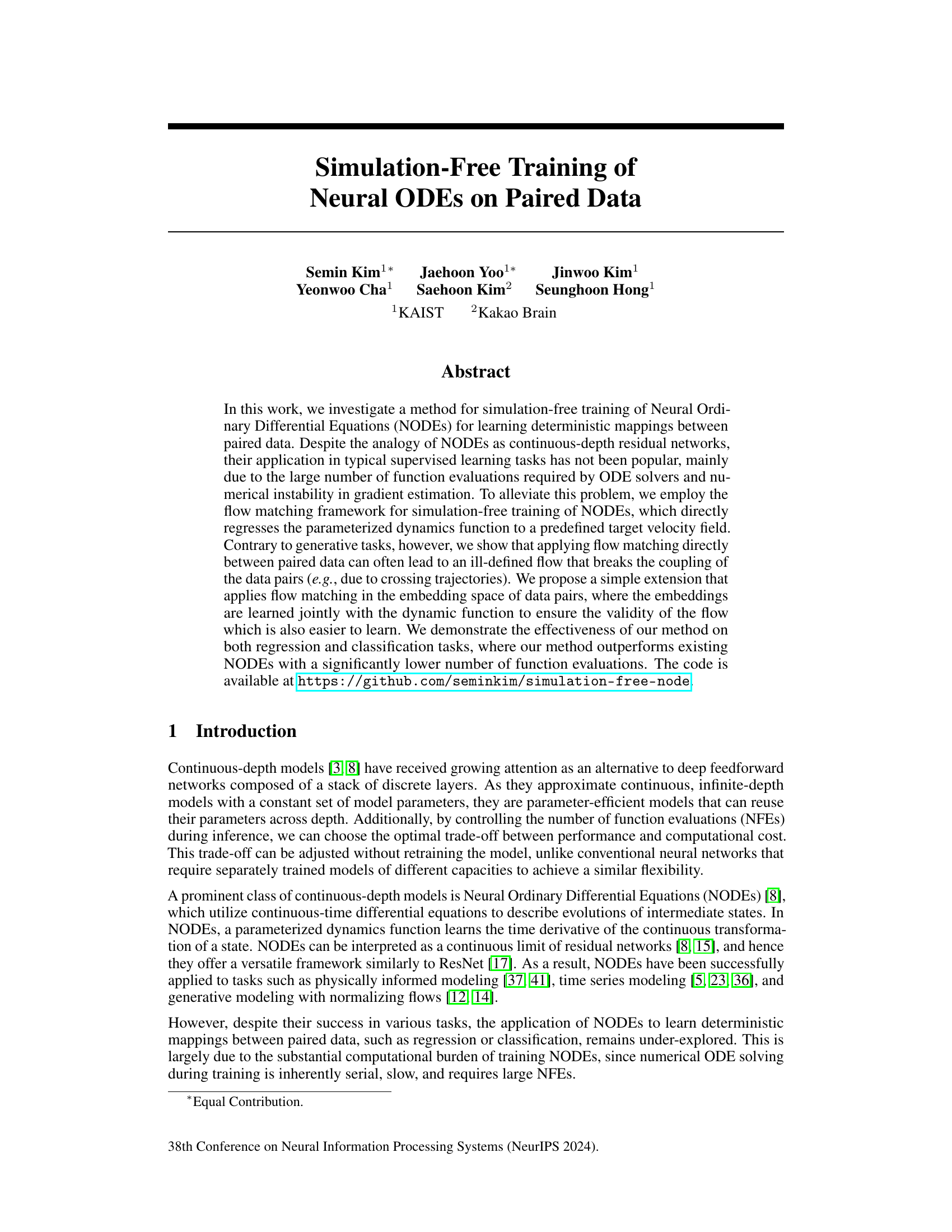
🔼 This figure compares the learned trajectories of four different methods on a simple deterministic regression task with four data pairs. The ground truth shows simple linear mappings between input and output pairs. A standard Neural ODE successfully learns the mapping but uses complex, computationally expensive trajectories. A flow matching approach, while efficient, fails to accurately pair inputs and outputs due to trajectory crossings. The proposed method, which uses embedding and flow matching, avoids crossings and correctly pairs inputs and outputs with minimal computational cost.
read the caption
Figure 1: Comparison of the learned trajectories. The final train loss (MSE) and training NFE are shown above each plot. (a) We consider deterministic regression task of four data pairs, each of which is represented by two circles (filled and empty circles) connected by dotted lines. (b) NODEs can correctly associate the pairs but through complex paths (solid lines) that require large NFEs. (c) Flow matching with linear velocity can greatly reduce the training NFEs by simulation-free training, but fails to associate the correct pairs due to the crossing trajectories induced by predefined dynamics. (d) The proposed method can alleviate the problems by learning the embeddings for data jointly with the flow matching.
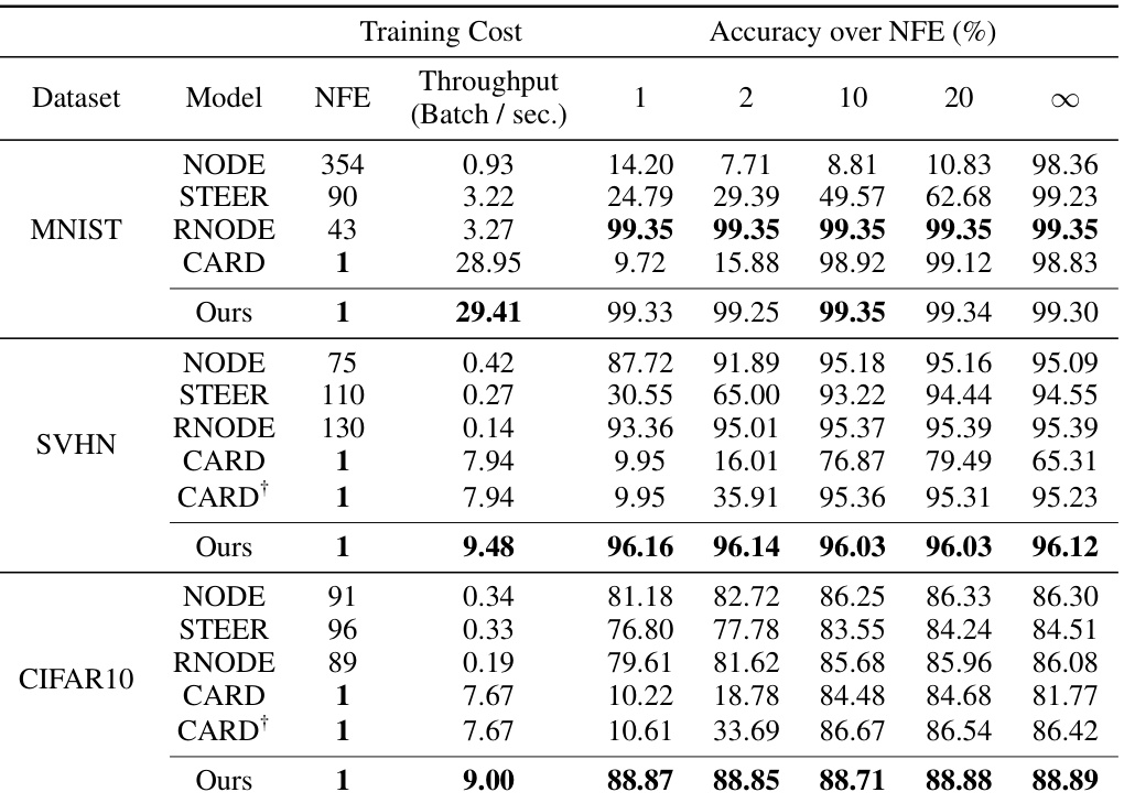
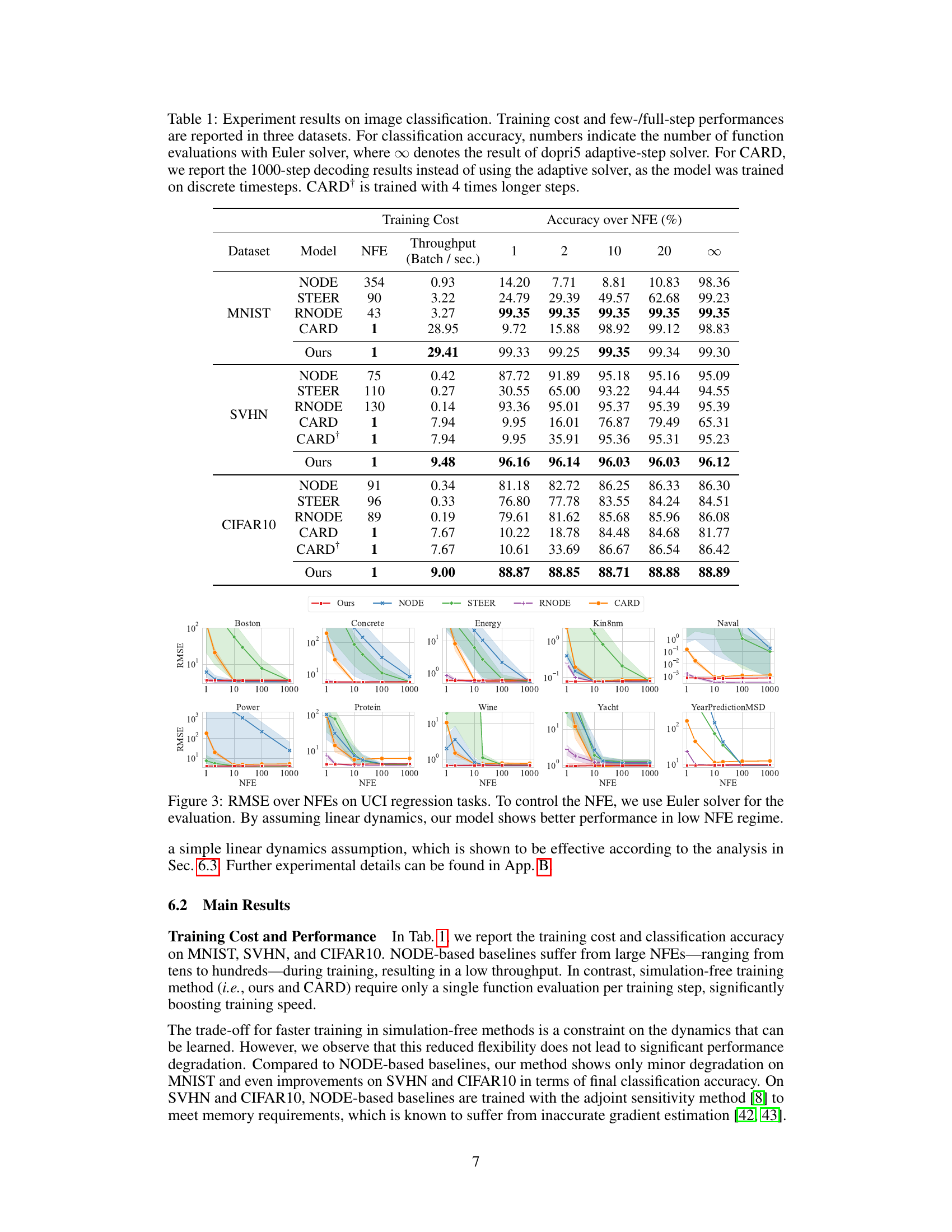
🔼 This table presents a comparison of different methods for image classification on three datasets: MNIST, SVHN, and CIFAR10. It shows the training cost (NFEs and throughput), and the classification accuracy achieved using different numbers of function evaluations (NFEs) with both the Euler solver (1, 2, 10, 20 NFEs) and the adaptive-step Dopri5 solver (∞ NFEs). The table also includes results for CARD, a diffusion-based model, trained with 1000 steps (and a variant trained with 4 times longer steps).
read the caption
Table 1: Experiment results on image classification. Training cost and few-/full-step performances are reported in three datasets. For classification accuracy, numbers indicate the number of function evaluations with Euler solver, where ∞ denotes the result of dopri5 adaptive-step solver. For CARD, we report the 1000-step decoding results instead of using the adaptive solver, as the model was trained on discrete timesteps. CARD† is trained with 4 times longer steps.
In-depth insights#
Sim-free NODE Training#
Simulation-free training of Neural Ordinary Differential Equations (NODEs) offers a compelling approach to learning deterministic mappings from data by directly regressing the dynamics function, thus circumventing the computationally expensive ODE solving traditionally required. The core challenge lies in ensuring that the learned dynamics remain well-behaved, avoiding issues like trajectory crossing that can arise from directly applying the flow matching framework to paired data. The proposed method cleverly addresses this by introducing learnable embeddings which transform the data into a space where a simple, predefined flow (e.g., linear) can produce valid and readily learnable trajectories. This embedding approach is crucial, maintaining data association while enabling efficient simulation-free training. The resulting method demonstrates improved efficiency, particularly in low-function evaluation scenarios, achieving competitive performance compared to traditional NODE methods and other simulation-free approaches.
Flow Matching Pitfalls#
Flow matching, while efficient for training continuous-depth models, presents pitfalls when applied to deterministic mappings between paired data. Directly applying flow matching can lead to ill-defined flows, particularly when the target velocity field is predefined. This is because the method often ignores the inherent coupling between input and output pairs. Consequently, crossing trajectories may arise in the data space, violating the underlying assumption of deterministic ODEs. These crossings cause errors and lead to incorrect associations between inputs and outputs. To mitigate these issues, learning embeddings jointly with the dynamic function is crucial. These embeddings map data pairs into a space where the predefined flow produces valid trajectories, avoiding the issue of trajectory crossings and enabling better performance, especially in low function evaluation scenarios. Therefore, a careful consideration of the data space and flow characteristics is necessary to successfully leverage flow matching for deterministic tasks.
Latent Space Training#
Latent space training, in the context of Neural Ordinary Differential Equations (NODEs), offers a powerful approach to address challenges in traditional NODE training. By learning embeddings of input data and labels in a shared latent space, this method effectively tackles the issue of trajectory crossings that often arise when applying flow matching directly to the raw data. The key advantage lies in separating the learning of data relationships from the learning of the dynamics function. Instead of directly regressing the dynamics function to a velocity field in raw data space, which can lead to poorly defined flows and inaccurate mappings, this method learns an embedding where a simple flow matching objective produces valid, non-crossing trajectories. This technique significantly reduces computational cost and improves learning stability. The embeddings themselves act as a regularizer, preventing trivial solutions and ensuring meaningful coupling between input and output. Furthermore, employing simple, linear flows within the latent space is often sufficient to achieve high performance, drastically lowering the number of function evaluations needed, both during training and inference. The simplicity of the latent space flow enhances few-step inference accuracy which is a significant improvement for real-time or resource-constrained applications. This approach elegantly combines the benefits of flow matching with the power of latent space representations for effective and efficient NODE training. Therefore, latent space training provides a promising direction for overcoming significant limitations of conventional NODE approaches for supervised learning tasks.
Low-NFE Regime#
The concept of a “Low-NFE Regime” in the context of Neural Ordinary Differential Equations (NODEs) is crucial because it highlights the trade-off between accuracy and computational efficiency. Reducing the number of function evaluations (NFEs) is paramount for deploying NODEs in resource-constrained environments or real-time applications where speed is critical. The authors explore this by comparing the performance of their proposed simulation-free training of NODEs with existing methods. Their method shows superior performance at lower NFEs, demonstrating its efficiency in this low-resource setting. This is particularly important for scenarios where the cost of computing ODE solutions becomes prohibitive, making their approach practically significant for deploying continuous-depth models in real-world applications. The results suggest that carefully designed methods focusing on efficient training and inference can unlock the full potential of NODEs for a wider range of tasks.
Future Research#
The authors suggest several promising avenues for future work. Extending the framework to handle more complex, nonlinear dynamics is a key area. While the current work focuses on linear dynamics for simplicity and efficiency, exploring learnable dynamics functions, possibly informed by Koopman operator theory, could unlock greater flexibility and applicability. Addressing the challenge of handling high-dimensional data more efficiently is also crucial. The current approach might struggle with very large datasets or complex input features. Incorporating techniques from dimensionality reduction or more efficient deep learning architectures could alleviate this. Finally, expanding the application domains to tackle diverse supervised learning tasks beyond regression and classification is important for demonstrating the broader utility of the proposed method. Investigating its potential for tasks such as time-series analysis, generative modeling, or physical modeling would be particularly insightful.
More visual insights#
More on figures

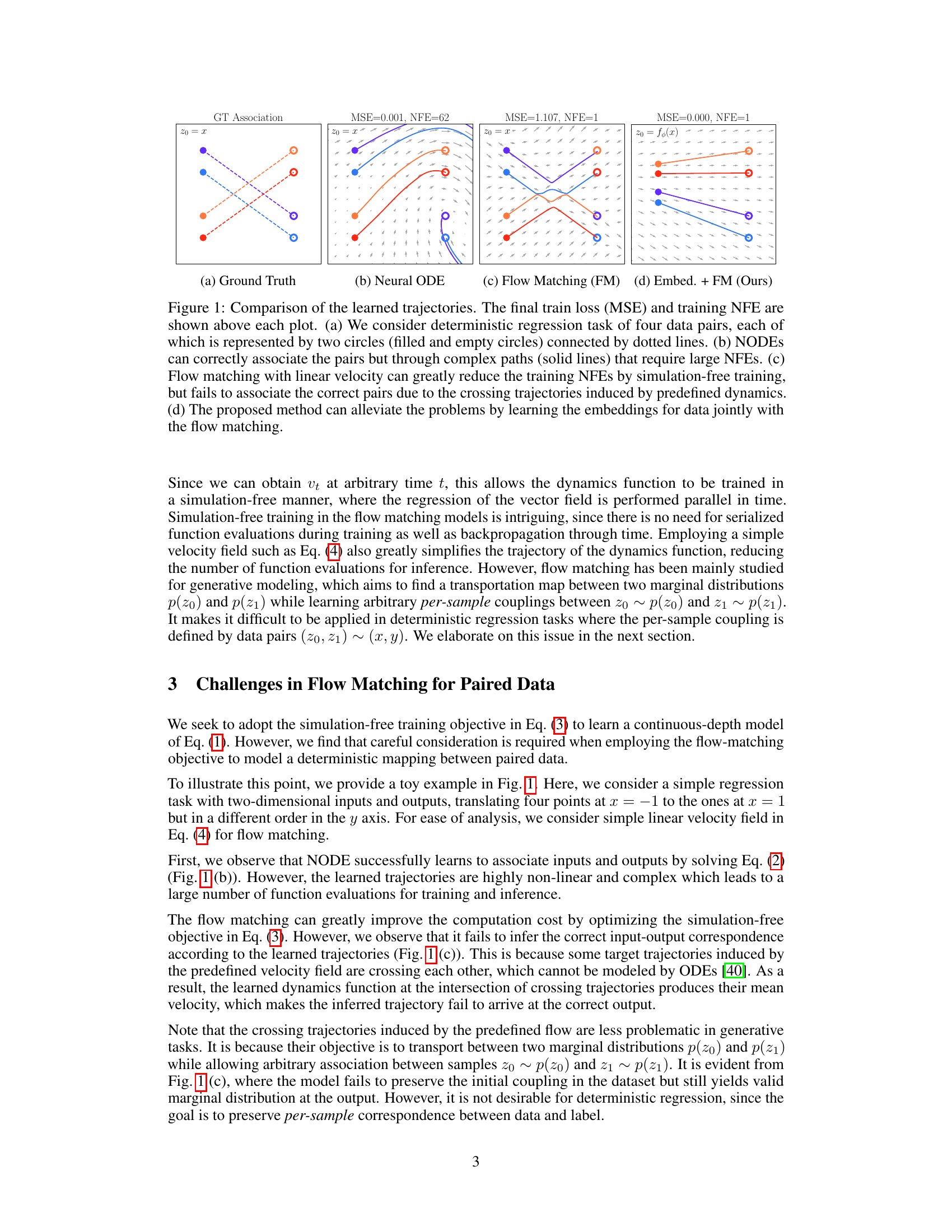
🔼 This figure illustrates the proposed framework for simulation-free training of Neural ODEs. It shows how data and labels are first encoded into an embedding space using separate encoders. In this embedding space, a predefined flow (dynamics) is applied to generate a trajectory that avoids the problematic crossing trajectories seen in the original data space. The embedding space is learned alongside the dynamic function, ensuring the validity of the flow. Finally, the label is decoded from the embedding space. This process greatly reduces the computational cost compared to standard training methods.
read the caption
Figure 2: An overview of our framework. We avoid the crossing trajectory problem in data space by introducing learnable encoders that project data and label to embedding space. In the learned embedding space, the presumed dynamics induce valid target velocity field.

🔼 This figure compares the root mean squared error (RMSE) achieved by different models on various UCI regression datasets as a function of the number of function evaluations (NFEs). The x-axis represents the NFEs, while the y-axis shows the RMSE. Each subplot corresponds to a different dataset. The lines represent the mean RMSE across multiple runs, and the shaded areas show the standard deviation. The figure demonstrates that the proposed method (Ours) achieves lower RMSE than the baseline methods (NODE, STEER, RNODE, CARD) especially when the number of NFEs is low, highlighting the efficiency of the proposed model, particularly when the computational resources are limited.
read the caption
Figure 3: RMSE over NFEs on UCI regression tasks. To control the NFE, we use Euler solver for the evaluation. By assuming linear dynamics, our model shows better performance in low NFE regime.

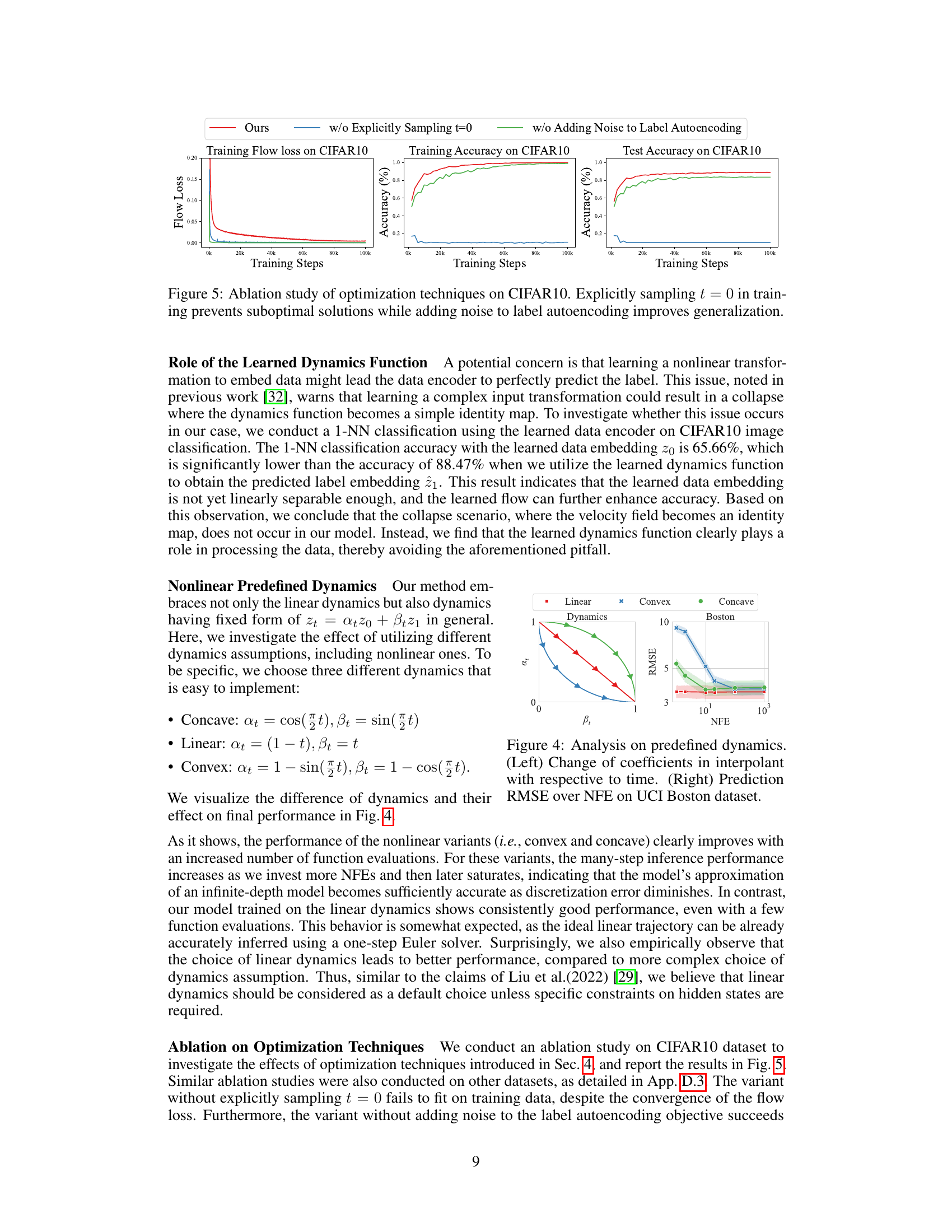
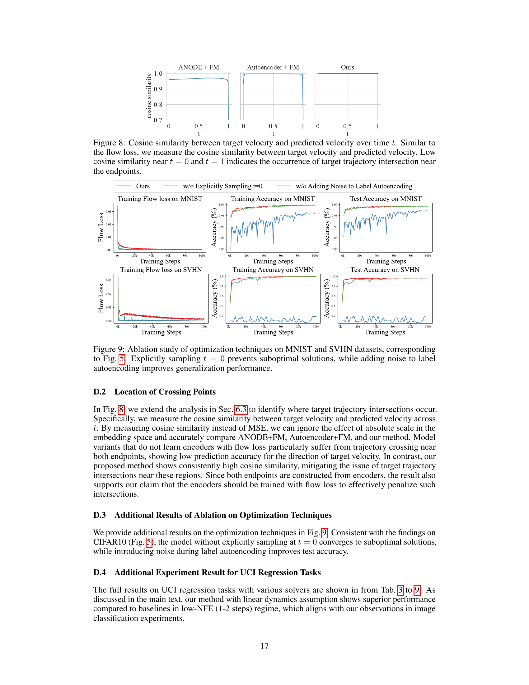
🔼 This ablation study investigates the impact of two optimization techniques on the performance of the proposed model for CIFAR10 image classification. The first technique is explicitly sampling t=0 during training. The second technique involves adding noise to the label autoencoding process. The results show that explicitly sampling t=0 prevents the model from converging to suboptimal solutions, leading to improved training and test accuracy. Adding noise to label autoencoding further enhances generalization performance. The figure visually represents these effects by plotting the training flow loss, training accuracy, and test accuracy across different training steps for the baseline model and the variants with each technique removed.
read the caption
Figure 5: Ablation study of optimization techniques on CIFAR10. Explicitly sampling t = 0 in training prevents suboptimal solutions while adding noise to label autoencoding improves generalization.
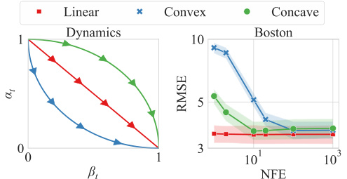
🔼 This figure analyzes the effect of different predefined dynamics on the model’s performance. The left panel shows the change in coefficients (αt and βt) of the interpolant zt = αtz0 + βtz1 over time t for three types of dynamics: linear, convex, and concave. The right panel presents the prediction Root Mean Squared Error (RMSE) versus the number of function evaluations (NFE) for the Boston housing dataset, using each of the three dynamics. It demonstrates how the choice of dynamics affects the model’s ability to achieve good performance with varying computational costs.
read the caption
Figure 4: Analysis on predefined dynamics. (Left) Change of coefficients in interpolant with respective to time. (Right) Prediction RMSE over NFE on UCI Boston dataset.

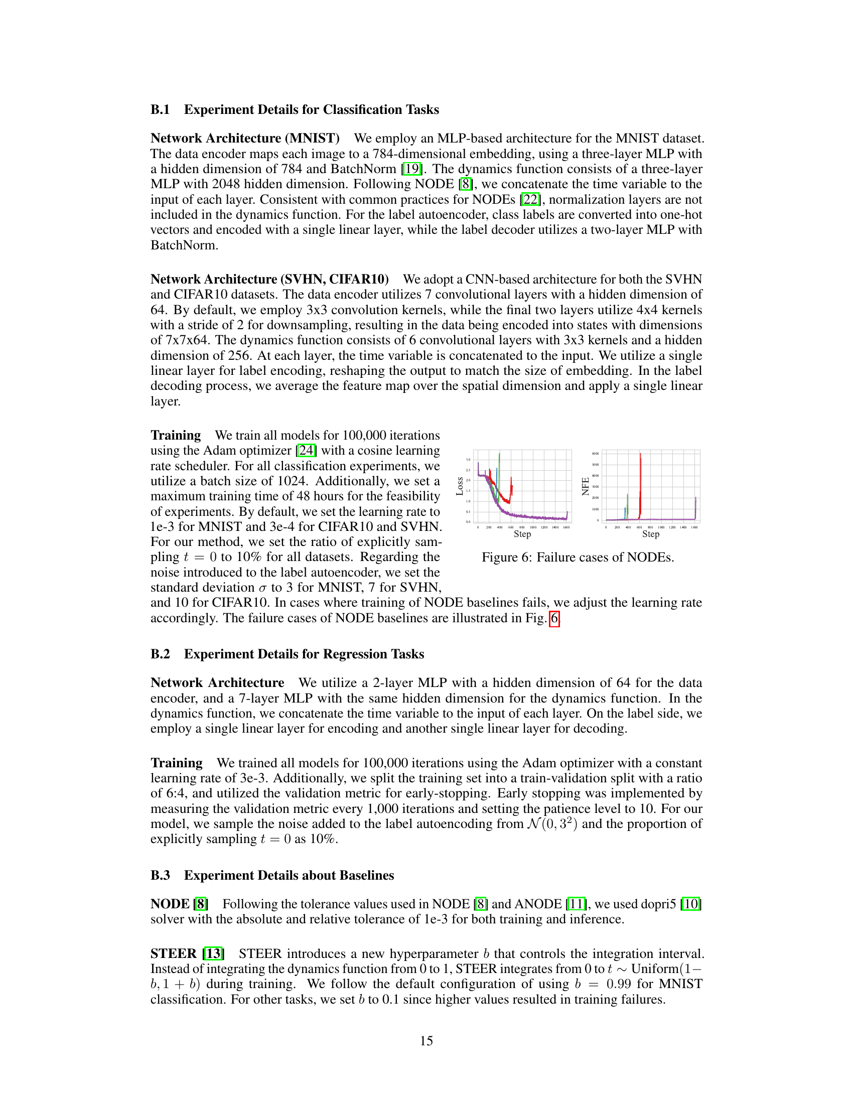
🔼 This figure shows examples where training of Neural Ordinary Differential Equations (NODEs) fails to converge. The x-axis represents the training step, the y-axis on the left shows the training loss, and the y-axis on the right shows the number of function evaluations (NFEs). The different colored lines represent different runs. The figure indicates that training NODEs can be unstable, failing to converge in multiple runs, despite adaptive step-size solvers.
read the caption
Figure 6: Failure cases of NODES.

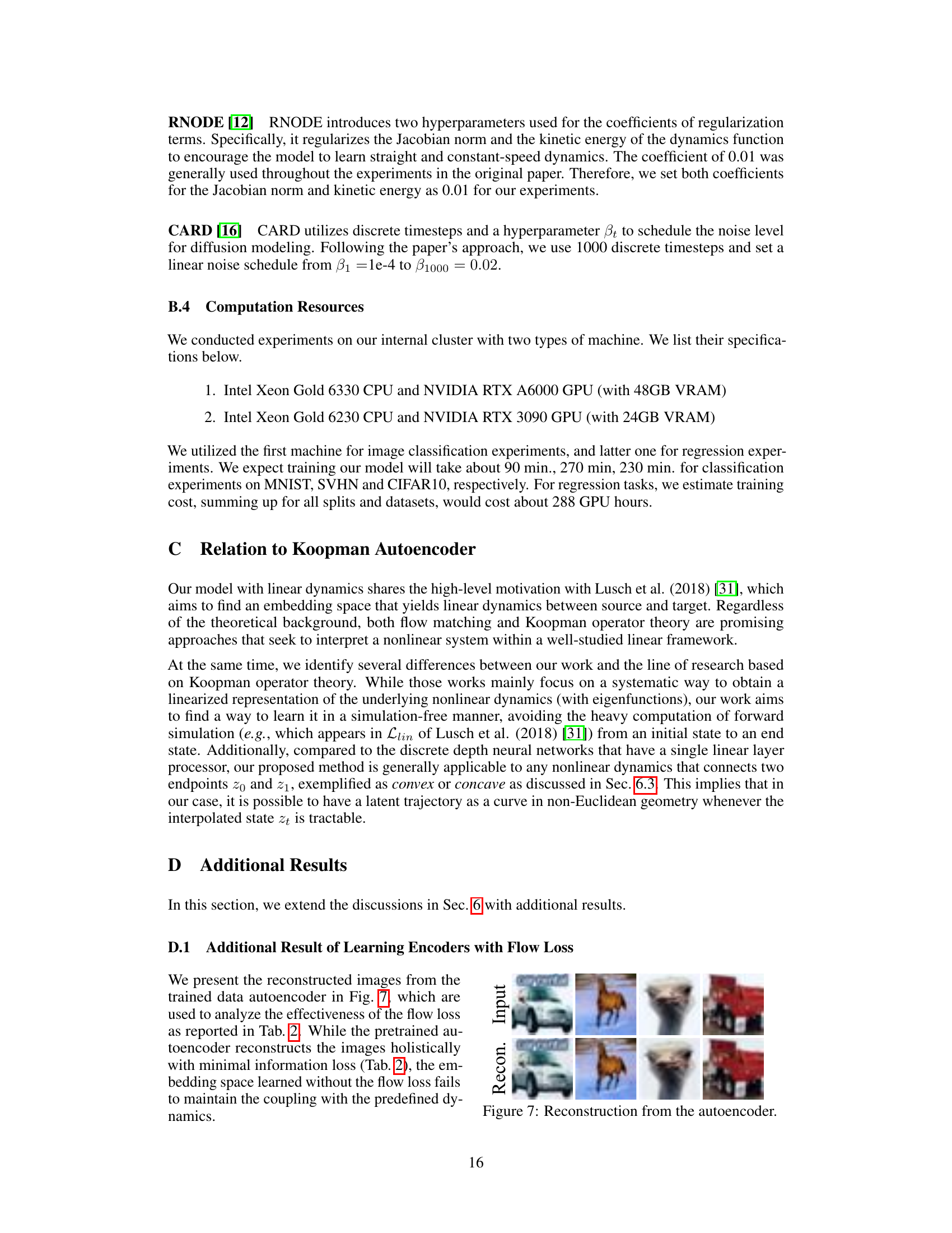
🔼 This figure shows the reconstruction of images from an autoencoder. The top row displays the input images, and the bottom row shows their reconstructions generated by the autoencoder. The purpose is to illustrate the quality of reconstruction achieved by the autoencoder used in the proposed method, specifically showing that the autoencoder trained without the flow loss fails to preserve the original coupling between data and label, resulting in a poor reconstruction. The images show that the reconstruction is quite good, suggesting that the autoencoder is effectively learning the relevant features of the input images.
read the caption
Figure 7: Reconstruction from the autoencoder.

🔼 This figure compares the learned trajectories of four different methods for a deterministic regression task. The ground truth shows four pairs of points directly connected. The Neural ODE method correctly connects the pairs but with complex and inefficient trajectories. Flow Matching, while efficient, causes trajectory crossings which is undesirable. The proposed ‘Embed.+FM’ method learns embeddings, avoiding crossings while maintaining efficiency.
read the caption
Figure 1: Comparison of the learned trajectories. The final train loss (MSE) and training NFE are shown above each plot. (a) We consider deterministic regression task of four data pairs, each of which is represented by two circles (filled and empty circles) connected by dotted lines. (b) NODEs can correctly associate the pairs but through complex paths (solid lines) that require large NFEs. (c) Flow matching with linear velocity can greatly reduce the training NFEs by simulation-free training, but fails to associate the correct pairs due to the crossing trajectories induced by predefined dynamics. (d) The proposed method can alleviate the problems by learning the embeddings for data jointly with the flow matching.
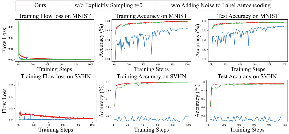
🔼 This figure shows the results of an ablation study conducted on the CIFAR10 dataset to investigate the effects of two optimization techniques: explicitly sampling t=0 during training and adding noise to the label autoencoding loss. The leftmost graph displays the training flow loss, showing that explicitly sampling t=0 prevents the model from converging to suboptimal solutions. The middle graph shows training accuracy, demonstrating that adding noise to the label autoencoding improves the model’s generalization ability. The rightmost graph displays test accuracy, confirming the benefit of adding noise to the label autoencoding for improved generalization performance. Overall, this ablation study highlights the importance of these optimization techniques in achieving optimal results.
read the caption
Figure 5: Ablation study of optimization techniques on CIFAR10. Explicitly sampling t = 0 in training prevents suboptimal solutions while adding noise to label autoencoding improves generalization.
More on tables

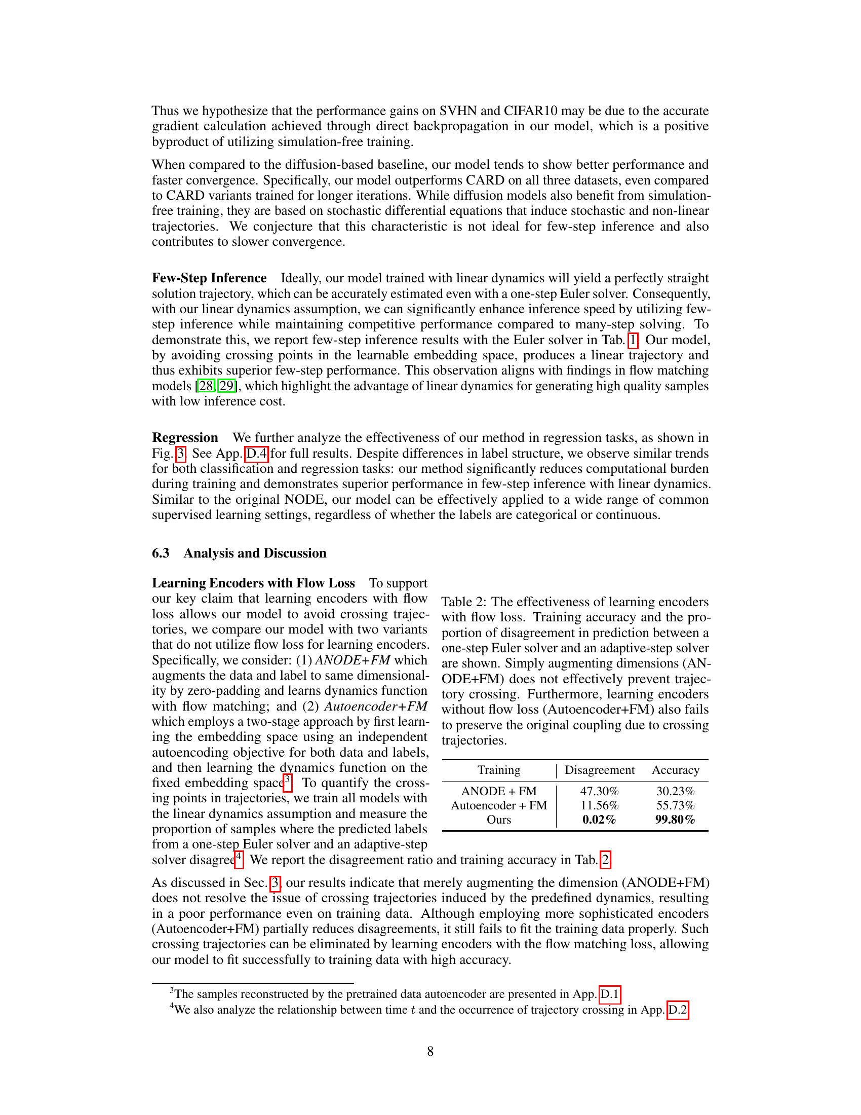
🔼 This table presents a comparison of three different methods for learning encoders in a continuous-depth model, focusing on the impact of using flow loss. The methods compared are ANODE+FM (augmenting dimensions and using flow matching), Autoencoder+FM (learning an embedding space with autoencoding and then applying flow matching), and the authors’ proposed method. The table shows the training accuracy and the percentage of disagreements between predictions made using a one-step Euler solver and an adaptive-step solver. The results demonstrate the effectiveness of the authors’ method in preventing trajectory crossing and achieving high accuracy.
read the caption
Table 2: The effectiveness of learning encoders with flow loss. Training accuracy and the proportion of disagreement in prediction between a one-step Euler solver and an adaptive-step solver are shown. Simply augmenting dimensions (ANODE+FM) does not effectively prevent trajectory crossing. Furthermore, learning encoders without flow loss (Autoencoder+FM) also fails to preserve the original coupling due to crossing trajectories.

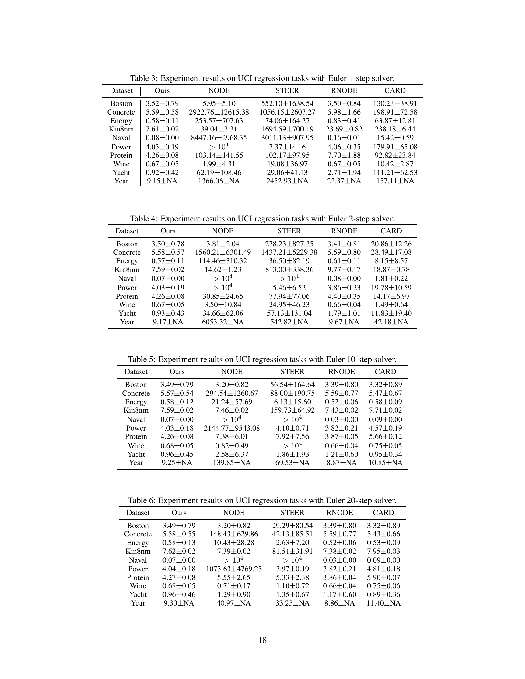
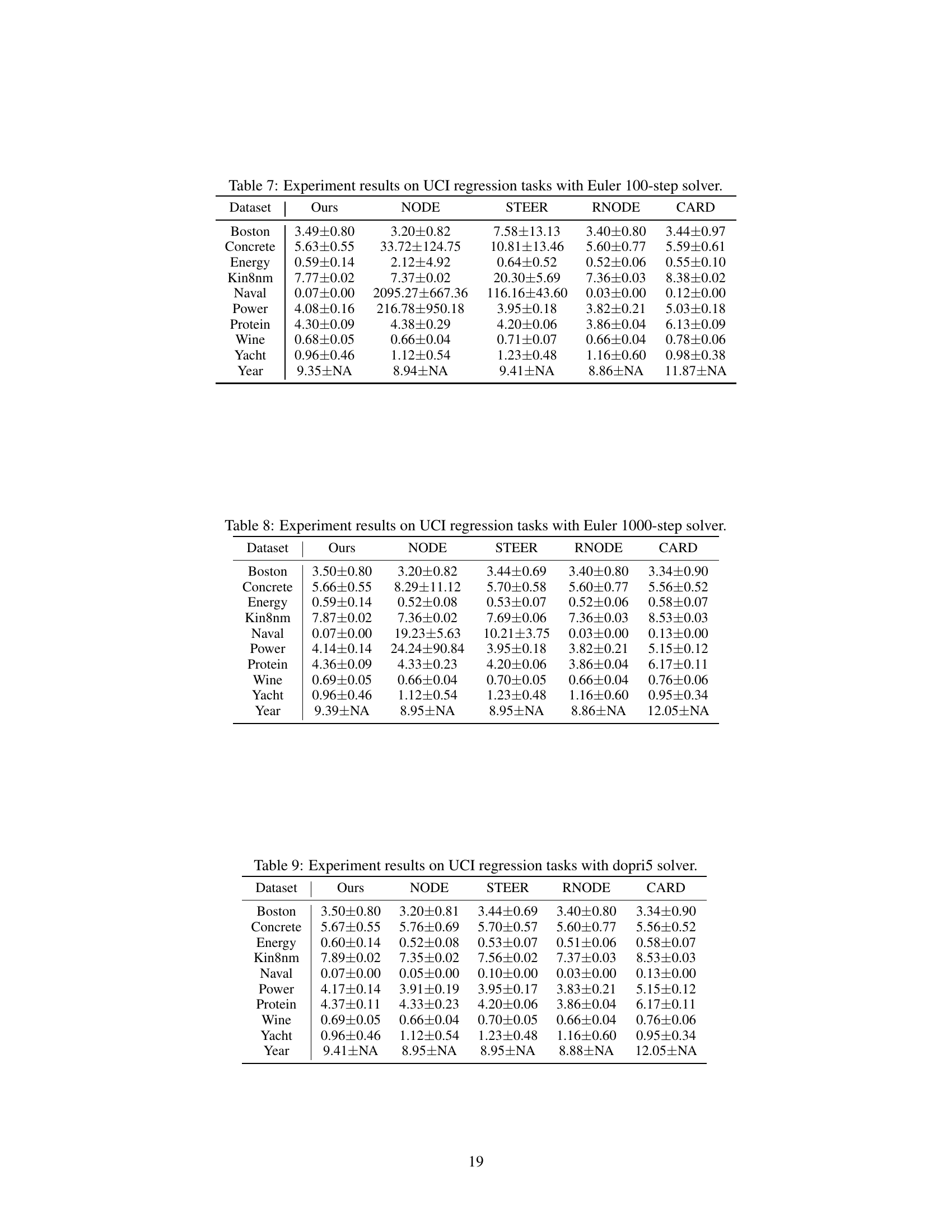
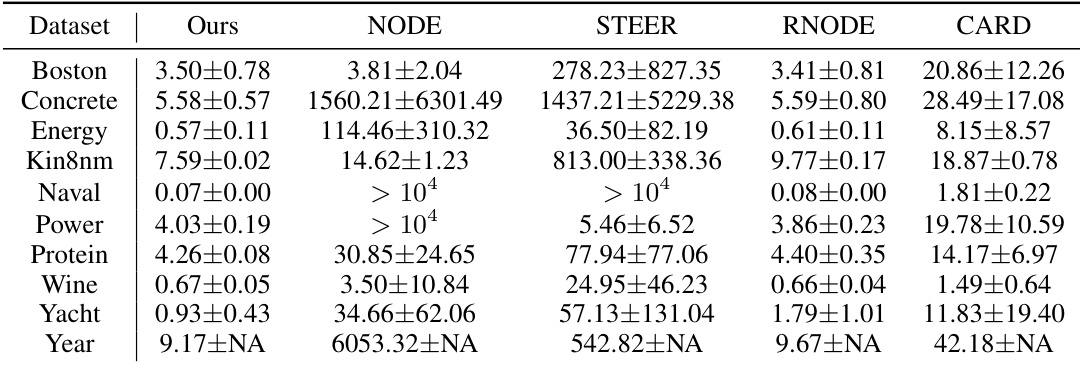
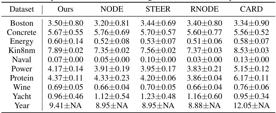
🔼 This table presents the results of experiments conducted on UCI regression datasets using the Euler method with a single step. It compares the performance of the proposed method (‘Ours’) against several baseline methods (NODE, STEER, RNODE, and CARD) in terms of Root Mean Square Error (RMSE). The RMSE values reflect the accuracy of each method in predicting the target variable, with lower values indicating better performance. The table showcases the relative performance of different methods using this specific experimental setup.
read the caption
Table 3: Experiment results on UCI regression tasks with Euler 1-step solver.
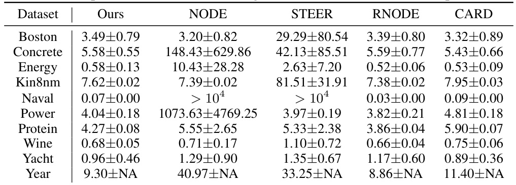
🔼 This table presents the results of UCI regression tasks using the Euler method with 2 steps. It compares the performance of the proposed method (‘Ours’) against several baseline methods (NODE, STEER, RNODE, and CARD) across various datasets. The metrics used are likely RMSE (root mean square error) values, with the plus/minus values representing some measure of uncertainty (e.g., standard deviation or confidence interval). The table highlights the relative performance of each method in terms of accuracy and computational efficiency. The ‘> 104’ entries likely indicate that the baseline methods required far more than 10,000 function evaluations.
read the caption
Table 4: Experiment results on UCI regression tasks with Euler 2-step solver.

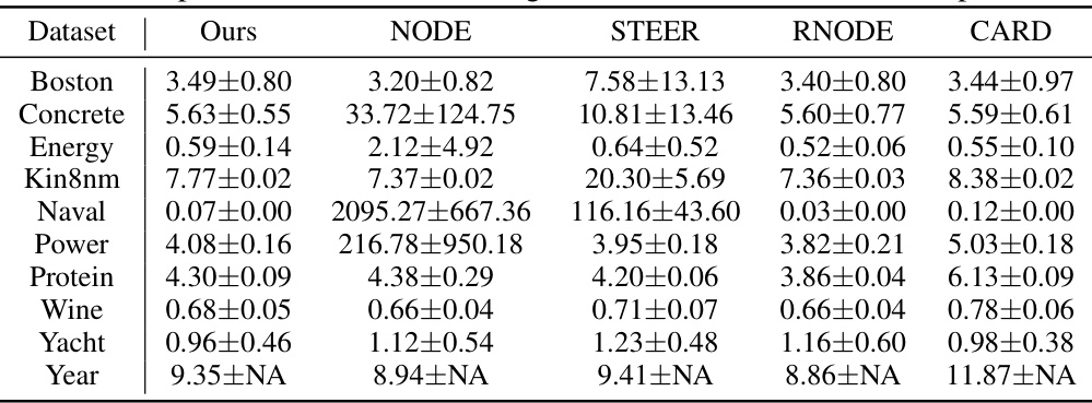
🔼 This table presents a comparison of different models’ performance on image classification tasks using three datasets: MNIST, SVHN, and CIFAR10. It shows training costs (NFEs and throughput), and classification accuracy at different numbers of function evaluations (NFEs) using both Euler and adaptive-step solvers. It highlights the trade-off between training efficiency and accuracy. The table also includes results for CARD, a model based on diffusion processes, comparing 1000-step decoding with other methods’ performance at various NFE.
read the caption
Table 1: Experiment results on image classification. Training cost and few-/full-step performances are reported in three datasets. For classification accuracy, numbers indicate the number of function evaluations with Euler solver, where ∞ denotes the result of dopri5 adaptive-step solver. For CARD, we report the 1000-step decoding results instead of using the adaptive solver, as the model was trained on discrete timesteps. CARD† is trained with 4 times longer steps.
🔼 This table presents a comparison of different methods for image classification on three datasets (MNIST, SVHN, CIFAR10). It shows the training cost (NFEs and throughput), and the classification accuracy achieved with varying numbers of function evaluations (NFEs) using both the Euler solver (few-step inference) and the dopri5 adaptive-step solver (full-step inference). The table also highlights the performance of CARD, a baseline method, trained with both standard and longer timesteps.
read the caption
Table 1: Experiment results on image classification. Training cost and few-/full-step performances are reported in three datasets. For classification accuracy, numbers indicate the number of function evaluations with Euler solver, where ∞ denotes the result of dopri5 adaptive-step solver. For CARD, we report the 1000-step decoding results instead of using the adaptive solver, as the model was trained on discrete timesteps. CARD† is trained with 4 times longer steps.
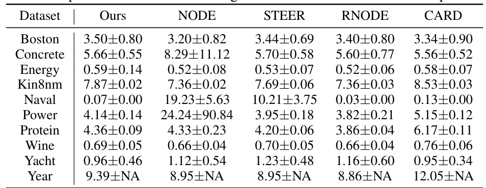
🔼 This table presents a comparison of different models on image classification tasks using three datasets: MNIST, SVHN, and CIFAR10. It shows the training cost (number of function evaluations (NFEs) and training throughput), and the classification accuracy achieved by each model at varying numbers of function evaluations (NFEs) during both few-step and full-step inference. The models compared include NODE, STEER, RNODE, CARD, and the proposed method. The table highlights the computational efficiency and accuracy of the proposed method, particularly in low-NFE settings.
read the caption
Table 1: Experiment results on image classification. Training cost and few-/full-step performances are reported in three datasets. For classification accuracy, numbers indicate the number of function evaluations with Euler solver, where ∞ denotes the result of dopri5 adaptive-step solver. For CARD, we report the 1000-step decoding results instead of using the adaptive solver, as the model was trained on discrete timesteps. CARD† is trained with 4 times longer steps.
🔼 This table presents a comparison of different models’ performance on image classification tasks using three datasets (MNIST, SVHN, CIFAR10). It shows training costs (NFEs and throughput), and classification accuracy at various numbers of function evaluations (NFEs) using both Euler and adaptive solvers. The table highlights the efficiency gains of the proposed simulation-free method compared to standard Neural ODEs and other baselines like STEER, RNODE, and CARD.
read the caption
Table 1: Experiment results on image classification. Training cost and few-/full-step performances are reported in three datasets. For classification accuracy, numbers indicate the number of function evaluations with Euler solver, where ∞ denotes the result of dopri5 adaptive-step solver. For CARD, we report the 1000-step decoding results instead of using the adaptive solver, as the model was trained on discrete timesteps. CARD† is trained with 4 times longer steps.
🔼 This table presents a comparison of different methods for image classification on three datasets: MNIST, SVHN, and CIFAR10. It shows the training cost (NFEs and throughput), and the accuracy achieved using different numbers of function evaluations (NFEs) for each method. The table highlights the efficiency gains from simulation-free training, particularly with the proposed method.
read the caption
Table 1: Experiment results on image classification. Training cost and few-/full-step performances are reported in three datasets. For classification accuracy, numbers indicate the number of function evaluations with Euler solver, where ∞ denotes the result of dopri5 adaptive-step solver. For CARD, we report the 1000-step decoding results instead of using the adaptive solver, as the model was trained on discrete timesteps. CARD† is trained with 4 times longer steps.
Full paper#
