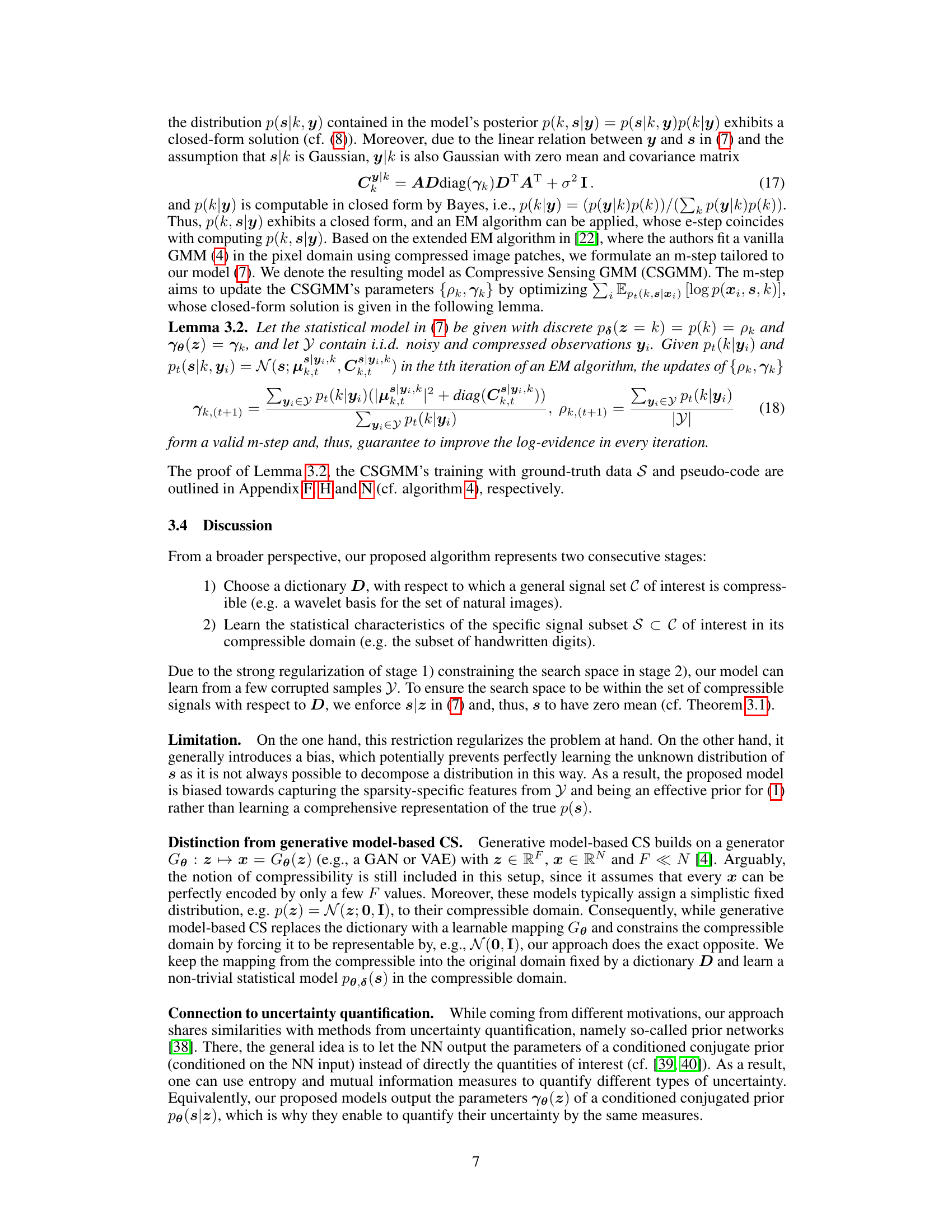
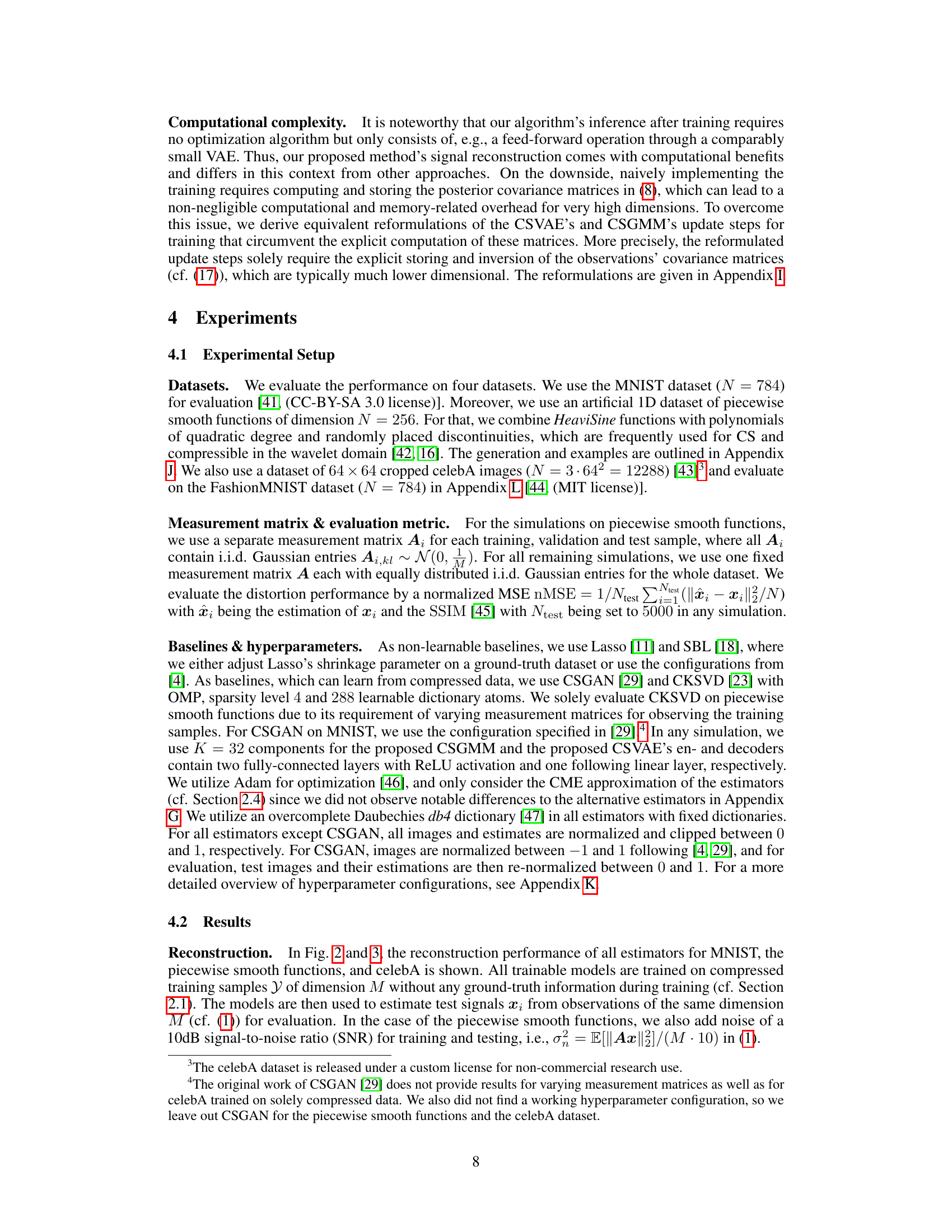
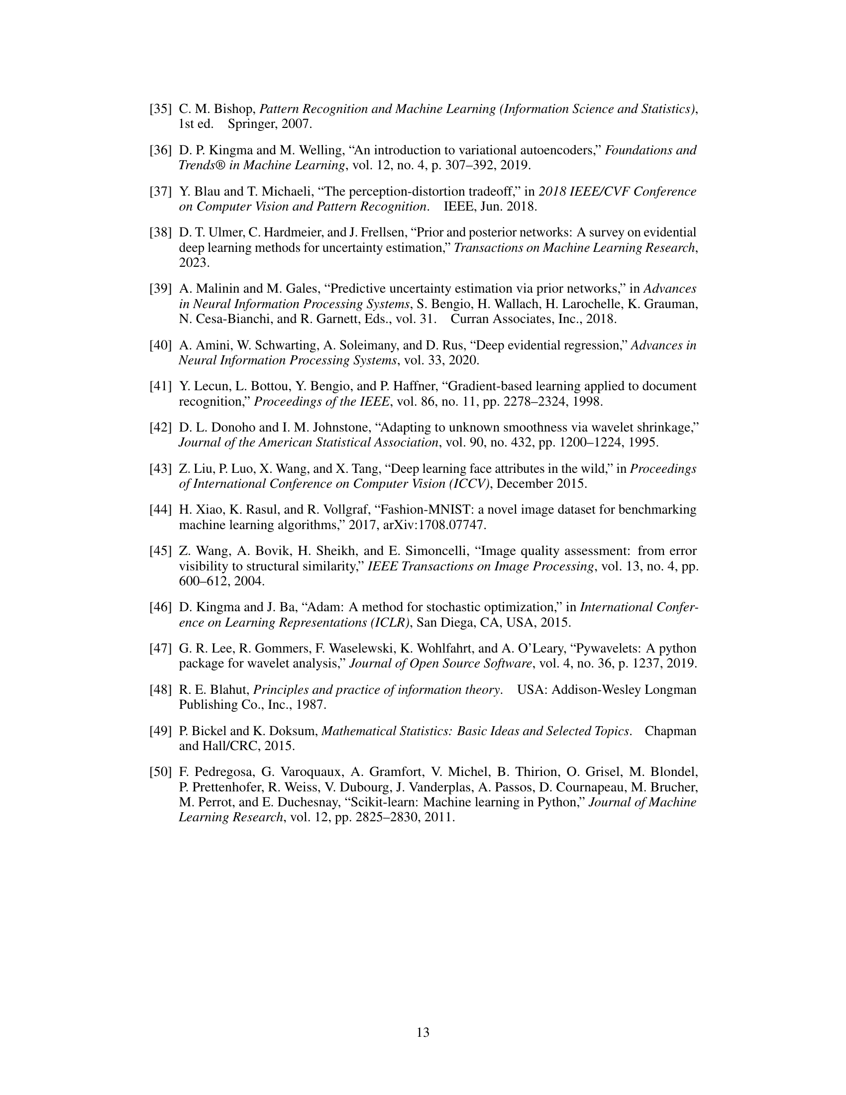
TL;DR#
Compressive sensing (CS) aims to reconstruct signals from incomplete measurements, but traditional methods struggle with noisy or limited data. Existing generative model-based CS approaches often require extensive ground-truth training data, limiting their applicability in real-world scenarios. This restricts their use in applications with limited access to ground-truth data like medical imaging and wireless communication. This paper addresses these issues.
The paper proposes a novel learnable prior called “Sparse Bayesian Generative Models,” combining ideas from dictionary-based CS and sparse Bayesian learning (SBL). This new method learns from a few compressed and noisy data samples, requiring no ground-truth data for training. It offers uncertainty quantification capabilities and a computationally efficient inference phase. Experiments show successful signal reconstruction across different signal types, outperforming existing techniques particularly when training data is scarce.
Key Takeaways#
Why does it matter?#
This paper is important because it introduces a novel approach to compressive sensing that addresses the limitations of existing methods. It is particularly relevant in scenarios with limited or noisy training data, opening new avenues for research in various applications such as medical imaging and wireless communication. The proposed model’s ability to learn from corrupted data and provide uncertainty quantification makes it a significant contribution to the field.
Visual Insights#

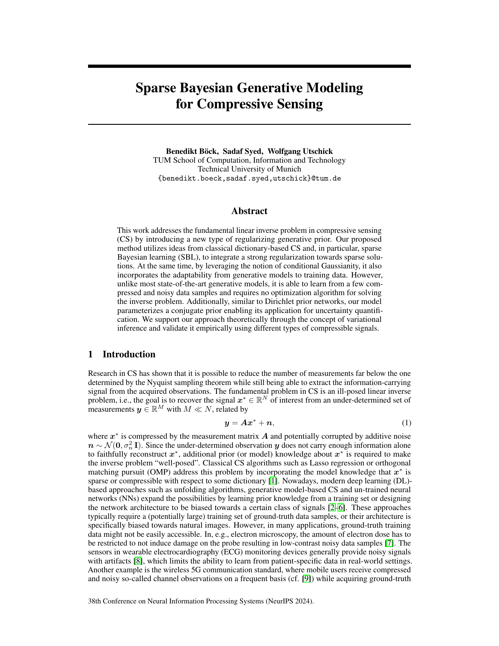
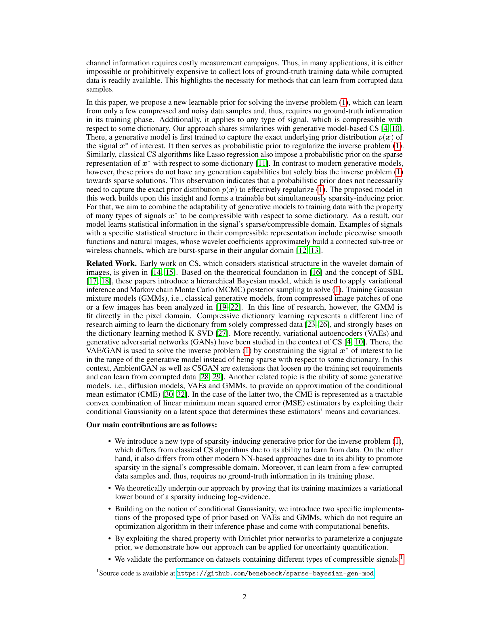
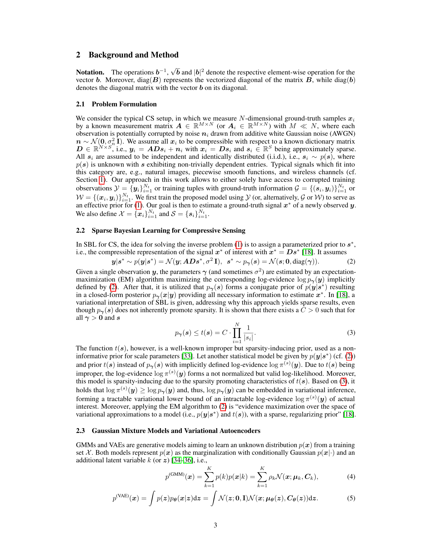
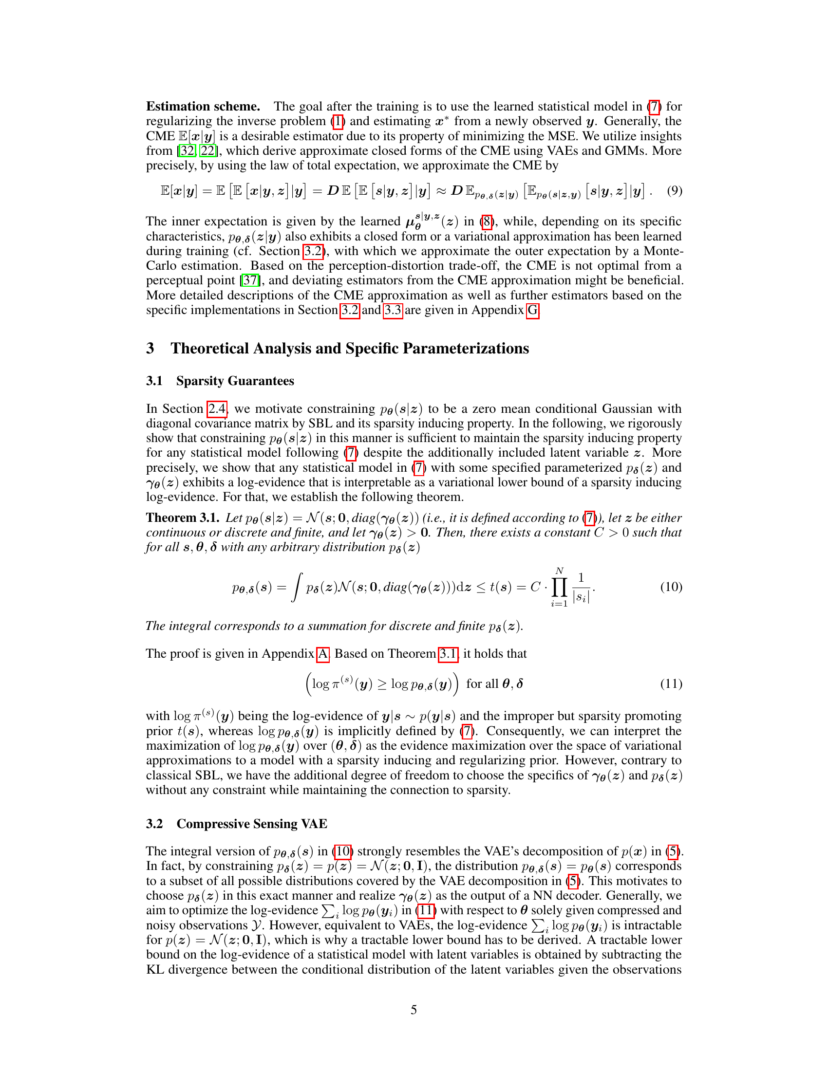
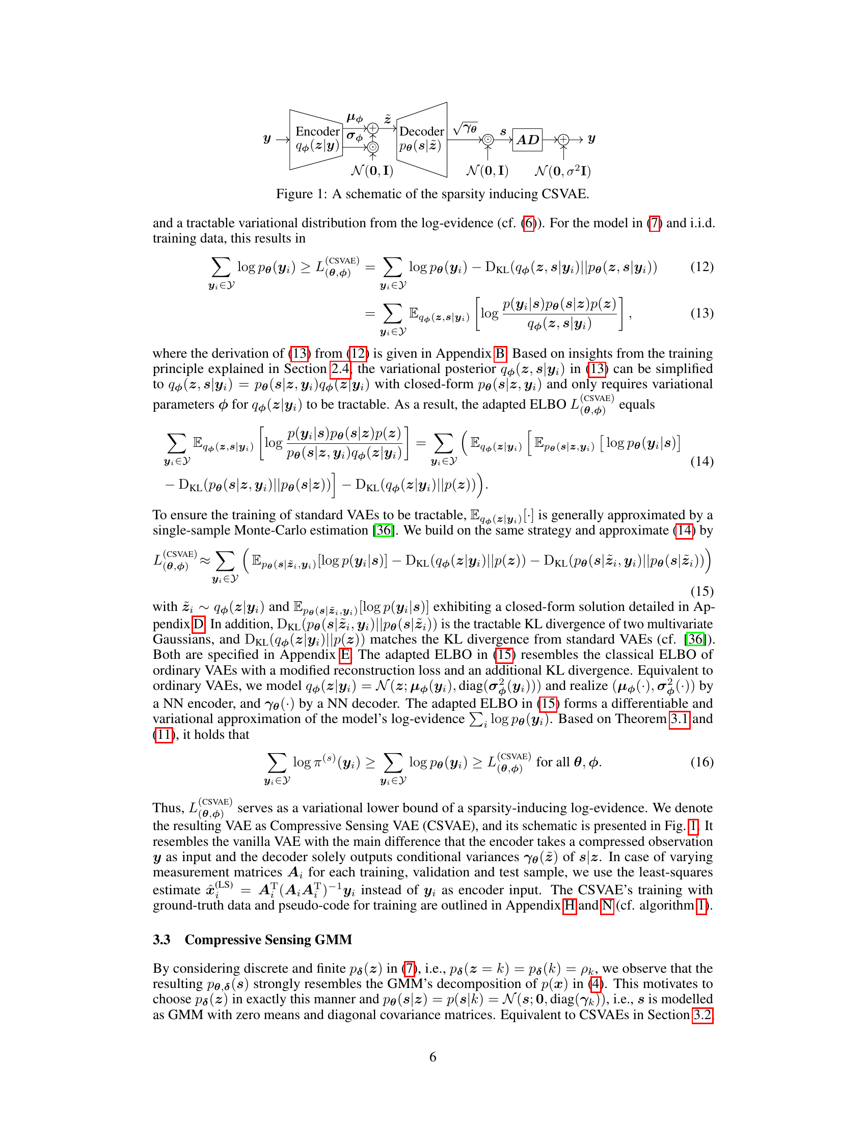
🔼 This figure shows a schematic of the sparsity-inducing CSVAE (Compressive Sensing Variational Autoencoder). The input is a compressed observation y, which is fed into an encoder that outputs the mean (μφ) and standard deviation (σφ) of a latent variable z. This latent variable is then sampled from a standard normal distribution N(0,I) and passed to a decoder that outputs the square root of the diagonal elements of the covariance matrix (√γθ) for the compressible representation s. This s is also sampled from a normal distribution N(0, I) and multiplied by the dictionary D and the measurement matrix A to generate a reconstruction of y which is corrupted by additive white Gaussian noise N(0,σ2I). The CSVAE is trained using variational inference to learn the parameters of the encoder and decoder such that the reconstruction closely matches the input y while promoting sparsity in s.
read the caption
Figure 1: A schematic of the sparsity inducing CSVAE.
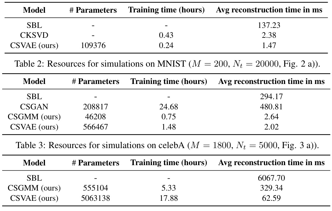
🔼 This table presents the computational resources required for running simulations on the celebA dataset using different models, including the proposed CSVAE and CSGMM. It shows the number of parameters, training time, and average reconstruction time for each model. The results highlight the efficiency of the proposed methods.
read the caption
Table 3: Resources for simulations on celebA (M = 1800, Nt = 5000, Fig. 3 a)).
In-depth insights#
Sparse Priors Learn#
The concept of “Sparse Priors Learn” suggests a research direction focusing on how sparse representations within machine learning models can be learned directly from data. Sparsity, meaning using only a small subset of available features or parameters, is valuable because it reduces computational costs, improves generalization, and enhances interpretability. A key challenge is to design algorithms that effectively learn these sparse priors from data, especially in scenarios with high dimensionality or limited training samples. This could involve novel Bayesian methods, regularized optimization techniques, or generative models tailored to sparse structures. Successful implementation would likely show improved performance in various learning tasks due to efficient use of resources and better generalization capabilities. This also relates to the field of compressive sensing, where acquiring fewer measurements than traditionally needed is possible by leveraging inherent sparsity in signals. An investigation into “Sparse Priors Learn” would likely explore the theoretical foundations, algorithm design, and practical applications of such methods across different machine learning domains.
Gen. Model Inference#
Generative model inference in the context of compressive sensing involves using a learned generative model to estimate the underlying signal from its compressed measurements. This approach offers several advantages. First, it leverages the power of deep learning to capture complex data distributions and relationships that might be missed by traditional methods. Second, generative models can provide uncertainty estimates associated with the recovered signal. Third, they offer a natural framework for handling noise and missing data. However, several crucial considerations arise in practical applications. Computational cost is a significant concern. Inference can be computationally demanding, especially for high-dimensional signals and complex generative models. Generalizability is also a major concern. A generative model trained on one specific type of signal may not perform well on other types of signals. Data requirements are another factor. Training a good generative model typically requires a large dataset of ground truth data, but real-world compressive sensing applications may lack this. This creates a tension between leveraging deep learning’s power and the constraints imposed by real world data limitations.
Variational Inference#
Variational inference (VI) is a powerful approximate inference technique commonly used when exact inference is intractable, particularly in complex probabilistic models. VI frames inference as an optimization problem, where we search for the simplest probability distribution that best approximates the true, often complex, posterior distribution. This approximation is typically achieved using a family of simpler distributions, such as Gaussians, that are parameterized and optimized to minimize a divergence measure (e.g. KL-divergence) from the true posterior. The core of VI lies in finding the optimal parameters of this approximating distribution, often through gradient-based optimization methods. A key advantage of VI is its scalability; it can handle large datasets and high-dimensional models where other techniques fail. However, the accuracy of VI relies heavily on the choice of the approximating family. If this family is poorly chosen, the approximation may be inaccurate or even misleading. Furthermore, assessing the quality of the approximation can be challenging, requiring careful consideration and possibly advanced diagnostic tools.
Compressible Signals#
The concept of “compressible signals” is crucial in compressive sensing (CS), forming the foundation for its ability to reconstruct signals from far fewer measurements than traditional methods require. Compressibility doesn’t mean a signal is inherently small; rather, it implies that the signal can be efficiently represented using a small number of coefficients in a specific domain, often achieved through transformations like wavelets or Fourier transforms. This sparsity, or near-sparsity, in the transformed domain is key. The efficiency of CS hinges on exploiting this compressibility: algorithms are designed to recover the sparse representation, and then the inverse transform yields the original signal. Different signal types exhibit varying degrees of compressibility depending on their inherent structure and the chosen transform. For instance, images often exhibit compressibility in the wavelet domain due to their piecewise smooth nature, while other signals might be sparse in the frequency domain. The choice of transform is thus critical to the success of CS for a particular signal type. Research into compressible signals extends to identifying and characterizing those structures that allow for efficient compression, paving the way for better CS algorithms and broader applications.
Future Research#
The paper’s ‘Future Research’ section could explore several promising avenues. Extending the model to handle more complex signal structures beyond those tested (e.g., incorporating temporal dependencies or non-linear relationships) is crucial for broader applicability. Investigating the sensitivity of the model to hyperparameter choices and developing more robust methods for hyperparameter optimization would strengthen the approach. A deeper theoretical analysis could focus on deriving tighter bounds for the log-evidence and exploring connections to other sparsity-inducing priors. Improving computational efficiency is essential, possibly through algorithmic optimizations or exploring alternative network architectures. Finally, a focus on uncertainty quantification techniques beyond entropy measures and applications in real-world scenarios will increase practical impact.
More visual insights#
More on figures

🔼 This figure presents the results of the experiments conducted to evaluate the performance of different algorithms on the MNIST dataset and a dataset of piecewise smooth functions. Subfigures (a) and (b) show the normalized mean squared error (nMSE) and structural similarity index (SSIM) for varying numbers of measurements (M) while keeping the number of training samples constant. Subfigures (c) and (d) show the same metrics but with a fixed number of measurements (M) and varying numbers of training samples (Nt). Subfigure (e) displays example reconstructions of MNIST digits. Subfigures (f) and (g) illustrate the performance on the piecewise smooth function dataset, with varying M and Nt respectively, and show nMSE results for signal-to-noise ratio (SNR) of 10dB. Subfigure (h) provides example reconstructions of the piecewise smooth functions. Finally, subfigure (i) compares the performance of the algorithms using different types of dictionaries.
read the caption
Figure 2: a) and b) nMSE and SSIM over M (Nt = 20000, MNIST), c) and d) nMSE and SSIM over Nt (M = 160, MNIST), e) exemplary reconstructed MNIST images (M = 200, Nt = 20000), f) nMSE over M (SNRdB = 10dB, Nt = 10000, piece-wise smooth fct.), g) nMSE over Nt (SNRdB = 10dB, M = 100, piece-wise smooth fct.), h) exemplary reconstructed piece-wise smooth fct. (M = 100, Nt = 1000), i) nMSE comparison of dictionaries (MNIST, M = 160, Nt = 20000).

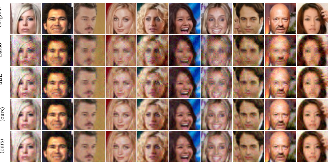
🔼 Figure 3 presents the performance evaluation results of different models on the CelebA dataset. The plots illustrate the nMSE and SSIM metrics against varying observation dimensions (M) and training sample sizes (Nt). Exemplar reconstructed CelebA images are shown to visualize the models’ performance. A histogram shows uncertainty quantification by displaying the differential entropy h(z|y) for the CSVAE trained only on compressed MNIST zeros. Finally, training and reconstruction times for the MNIST dataset are provided.
read the caption
Figure 3: a) and b) nMSE and SSIM over M (Nt = 5000), c) and d) nMSE and SSIM over Nt (M = 1800), e) exemplary reconstructed celebA images (M = 2700, Nt = 5000), f) histogram of h(z|y) for compressed test MNIST images of digits 0, 1 and 7, where the CSVAE is trained on compressed zeros, g) training and reconstruction time for MNIST (M = 200, Nt = 20000).

🔼 This figure displays six example signals from a 1D dataset of piecewise smooth functions. These signals are used in the paper’s experiments to evaluate the proposed algorithm’s performance. The piecewise smooth nature of the functions is evident in the plots, exhibiting regions of relative smoothness interspersed with sharp transitions or discontinuities.
read the caption
Figure 4: Exemplary signals within the 1D dataset of piecewise smooth functions.
🔼 This figure displays the normalized mean squared error (nMSE) and structural similarity index (SSIM) for different models on the MNIST dataset and a dataset of piecewise smooth functions. Subfigures (a) and (b) show the performance with a varying number of measurements (M) and a fixed number of training samples (Nt), while subfigures (c) and (d) show the opposite, keeping M fixed and varying Nt. Subfigure (e) provides example reconstructions of MNIST digits. Subfigures (f) and (g) show the results on the piecewise smooth functions, and subfigure (h) provides example reconstructions. Finally, subfigure (i) compares the performance with various dictionaries.
read the caption
Figure 2: a) and b) nMSE and SSIM over M (N₁ = 20000, MNIST), c) and d) nMSE and SSIM over Nt (M = 160, MNIST), e) exemplary reconstructed MNIST images (M = 200, Nt = 20000), f) nMSE over M (SNRdB = 10dB, Nt = 10000, piece-wise smooth fct.), g) nMSE over Nt (SNRdB = 10dB, M = 100, piece-wise smooth fct.), h) exemplary reconstructed piece-wise smooth fct. (M = 100, Nt = 1000), i) nMSE comparison of dictionaries (MNIST, M = 160, Nt = 20000).

🔼 This figure compares the reconstruction results of MNIST images using different models. Subfigure (a) shows reconstructions from models trained only on compressed data without ground truth. Subfigure (b) shows reconstructions from models trained with ground truth data (either the compressible representation or the original image). The comparison highlights the impact of having ground truth during model training on the accuracy of the reconstruction. Each row represents a different model (SBL, CSGAN, CSGMM, and CSVAE), and each column shows a different image.
read the caption
Figure 7: Exemplary reconstructed MNIST images for M = 200, Nt = 20000 from a) models, which are solely trained on compressed data (with observations of dimension M), and b) models, which are trained on ground truth data.

🔼 This figure displays exemplary reconstructed images from the FashionMNIST dataset using various methods. The original images are shown for comparison alongside reconstructions generated by Lasso, SBL, CSGAN, CSVAE, and CSGMM. The purpose is to visually demonstrate the comparative performance of the different algorithms in reconstructing detailed features of the clothing items.
read the caption
Figure 8: Exemplary reconstructed FashionMNIST images (M = 200, Nt = 20000, Fig. 6 g), h)).

🔼 This figure shows ten example signals from the one-dimensional dataset of piecewise smooth functions used in the paper’s experiments. Each signal is a curve that demonstrates piecewise smoothness, meaning it consists of smooth segments connected with discontinuities. The signals are designed to be compressible, with statistical structure in their wavelet domain. This dataset is used to evaluate the performance of the proposed model and compare it with baseline methods for compressive sensing.
read the caption
Figure 4: Exemplary signals within the 1D dataset of piecewise smooth functions.

🔼 This figure displays example images reconstructed using different methods: Original, Lasso, SBL, CSGAN, CSVAE (ours), and CSGMM (ours). The parameters used for reconstruction were M = 160 and Nt = 20000. The figure visually demonstrates the quality of reconstruction achieved by each method, allowing for a qualitative comparison of their performance on MNIST image data. The quality of the reconstructed images from the original and the proposed method is similar, whereas the other reconstruction methods provide lower-quality outputs.
read the caption
Figure 10: Exemplary reconstructed MNIST images (M = 160, Nt = 20000, Fig. 2 a))
🔼 The figure shows the performance of different compressive sensing methods on MNIST and piecewise smooth function datasets. Subfigures (a) and (b) illustrate nMSE and SSIM versus the number of measurements (M) for a fixed number of training samples (Nt = 20000) on the MNIST dataset. Subfigures (c) and (d) show the same metrics but with a fixed M and varying Nt. Subfigure (e) displays example reconstructed MNIST images. Subfigures (f) and (g) show the results for the piecewise smooth function dataset with varying M and Nt, respectively, and include added noise. Subfigure (h) provides example reconstructions. Finally, subfigure (i) compares the performance of different dictionaries.
read the caption
Figure 2: a) and b) nMSE and SSIM over M (Nt = 20000, MNIST), c) and d) nMSE and SSIM over Nt (M = 160, MNIST), e) exemplary reconstructed MNIST images (M = 200, Nt = 20000), f) nMSE over M (SNRdB = 10dB, Nt = 10000, piece-wise smooth fct.), g) nMSE over Nt (SNRdB = 10dB, M = 100, piece-wise smooth fct.), h) exemplary reconstructed piece-wise smooth fct. (M = 100, Nt = 1000), i) nMSE comparison of dictionaries (MNIST, M = 160, Nt = 20000).
Full paper#
